1. Introduction
The following vignette aims at documenting and illustrating workflows
for producing PK ratio plots using the tlf-Library.
This vignette focuses PK ratio plots examples. Detailed documentation
on typical tlf workflow, use of
AgregationSummary, DataMapping,
PlotConfiguration, and Theme can be found in
vignette("tlf-workflow").
2. Illustration of basic PK ratio plots
2.1. Data
The data showed in the sequel is available at the following path:
system.file("extdata", "test-data.csv", package = "tlf").
In the code below, the data is loaded and assigned to
pkRatioData.
# Load example
pkRatioData <- read.csv(
  system.file("extdata", "test-data.csv", package = "tlf"),
  stringsAsFactors = FALSE
)

# pkRatioData
knitr::kable(utils::head(pkRatioData), digits = 2)| ID | Age | Obs | Pred | Ratio | AgeBin | Sex | Country | SD |
|---|---|---|---|---|---|---|---|---|
| 1 | 48 | 4.00 | 2.90 | 0.72 | Adults | Male | Canada | 0.69 |
| 2 | 36 | 4.40 | 5.75 | 1.31 | Adults | Male | Canada | 0.19 |
| 3 | 52 | 2.80 | 2.70 | 0.96 | Adults | Male | Canada | 0.98 |
| 4 | 47 | 3.75 | 3.05 | 0.81 | Adults | Male | Canada | 0.59 |
| 5 | 0 | 1.95 | 5.25 | 2.69 | Peds | Male | Canada | 0.44 |
| 6 | 48 | 2.45 | 5.30 | 2.16 | Adults | Male | Canada | 0.07 |
A list of information about pkRatioData can be provided
through metaData.
knitr::kable(data.frame(
  Variable = c("Age", "Obs", "Pred", "Ratio"),
  Dimension = c("Age", "Clearance", "Clearance", "Ratio"),
  Unit = c("yrs", "dL/h/kg", "dL/h/kg", "")
))| Variable | Dimension | Unit |
|---|---|---|
| Age | Age | yrs |
| Obs | Clearance | dL/h/kg |
| Pred | Clearance | dL/h/kg |
| Ratio | Ratio |
2.2. plotPKRatio
The function plotting PK ratios is: plotPKRatio(). Basic
documentation of the function can be found using:
?plotPKRatio. The typical usage of this function is:
plotPKRatio(data, metaData = NULL, dataMapping = NULL, plotConfiguration = NULL).
The output of the function is a ggplot object. It can be
seen from this usage that only data is a necessary input.
Default set ups are used for metaData,
dataMapping and plotConfiguration within the
call of plotPKRatio. For instance, if
dataMapping is not provided, smart mapping will check if
data contains "x" and "y" columns. If the
data has only two columns not named "x" and
"y", it will assume the first one should be plot in x-axis
and the second in y-axis. Then, PKRatioPlotConfiguration is
initialized if not provided, defining a standard configuration with
PK Ratio Plot as title, the current date as subtitle and
using predefined fonts as defined by the current theme.
2.3. Minimal example
The minimal example can work using directly the function
plotPKRatio(data = pkRatioData[, c("Age", "Ratio")]).
plotPKRatio(data = pkRatioData[, c("Age", "Ratio")])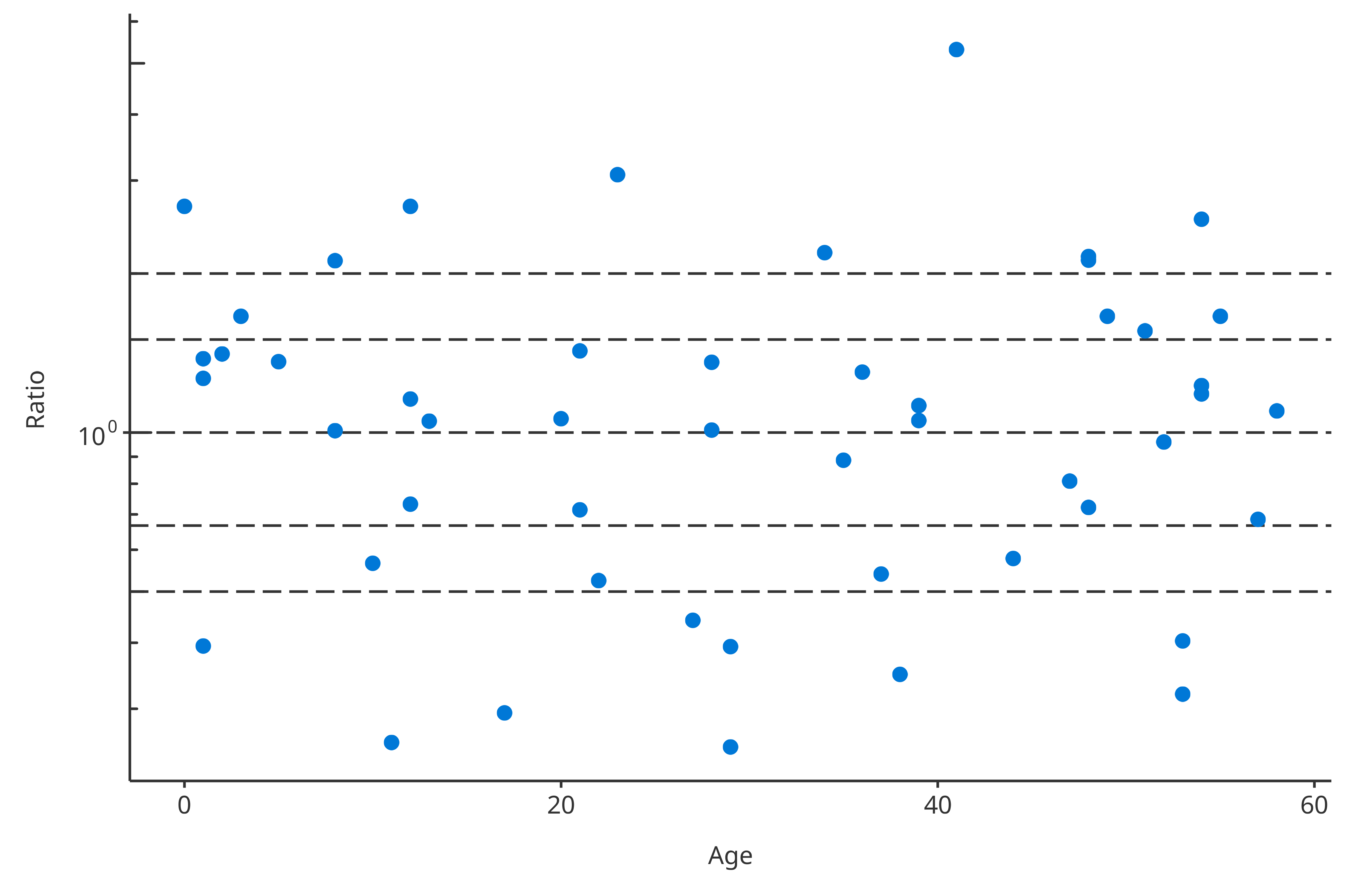
2.4. Examples with dataMapping
For PK ratio, the dataMapping class
PKRatioDataMapping includes 4 fields: x,
y, groupMapping and lines.
x and y define which variables from the data
will be plotted in X- and Y-axes, groupMapping is a class
mapping which aesthetic property will split which variables, and
lines defines horizontal lines performed in PK ratio
plots.
2.4.1 groupMapping
Some variables can be used to cluster the data. To this end,
PKRatioDataMapping objects include GroupMapping
objects that can define how to cluster based on a variable or a
data.frame. As illustrated below, most of the time, the direct input of
color and shape is faster to define such
objects. Consequently, the following examples are identical:
# Two-step process
colorMapping <- GroupMapping$new(color = "Sex")
dataMappingA <- PKRatioDataMapping$new(
x = "Age",
y = "Ratio",
groupMapping = colorMapping
)
print(dataMappingA$groupMapping$color$label)
#> [1] "Sex"
# One-step process
dataMappingB <- PKRatioDataMapping$new(
x = "Age",
y = "Ratio",
color = "Sex"
)
print(dataMappingB$groupMapping$color$label)
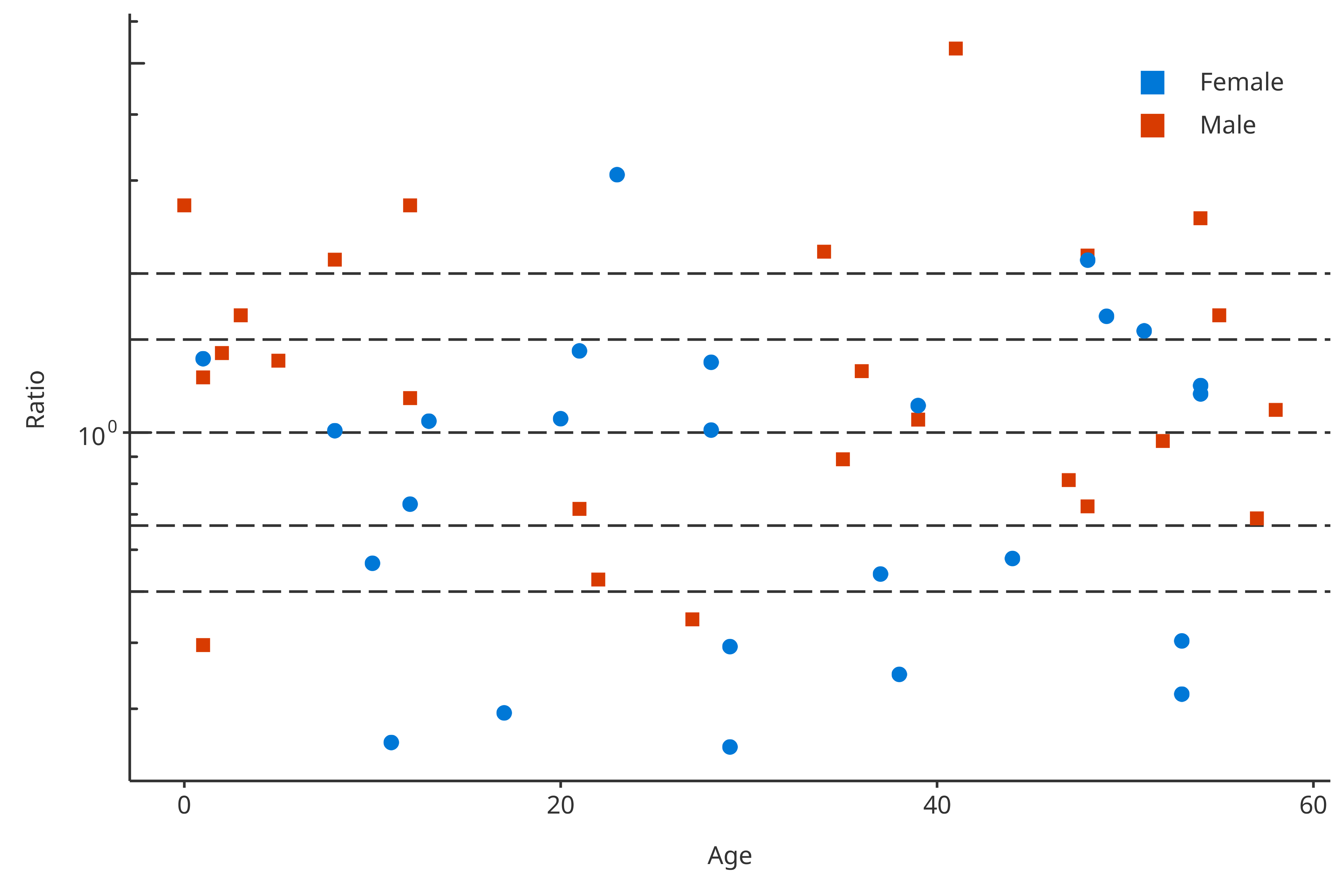
#> [1] "Sex"Then, in this example, plotPKRatio can use the
groupMapping to split the data by “Gender” and associate different
colors to each “Gender”:
plotPKRatio(
  data = pkRatioData,
  dataMapping = dataMappingB
)
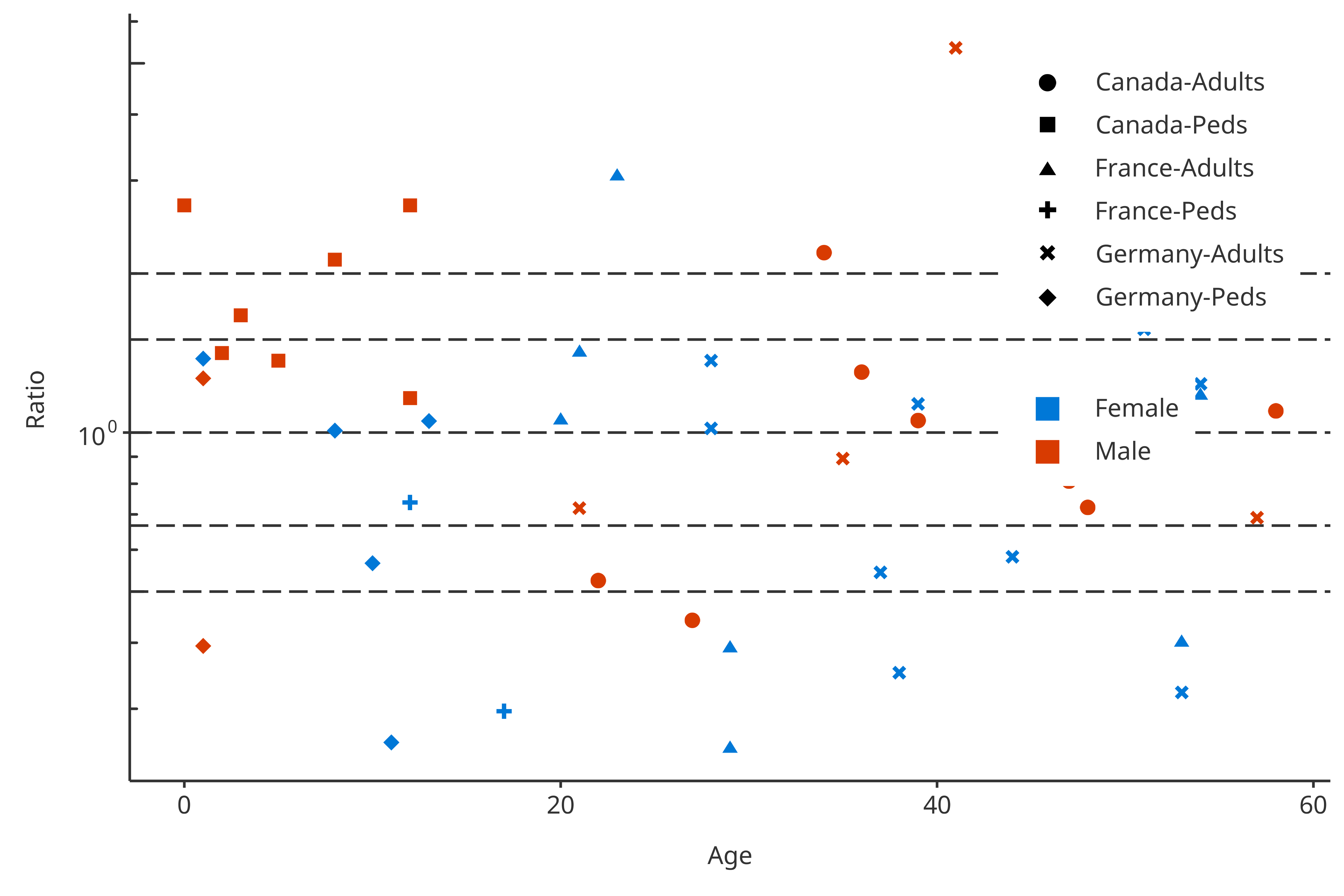
Multiple groupMappings can be performed for PK ratio: data can be
regrouped by color, shape and/or
size. The next example uses 2 groups in the groupMapping:
One group splits “Gender” by color, the other splits
shape by “Amount” and “Compound”.
dataMapping2groups <- PKRatioDataMapping$new(
  x = "Age",
  y = "Ratio",
  color = "Sex",
  shape = c("Country", "AgeBin")
)
plotPKRatio(
  data = pkRatioData,
  dataMapping = dataMapping2groups
)
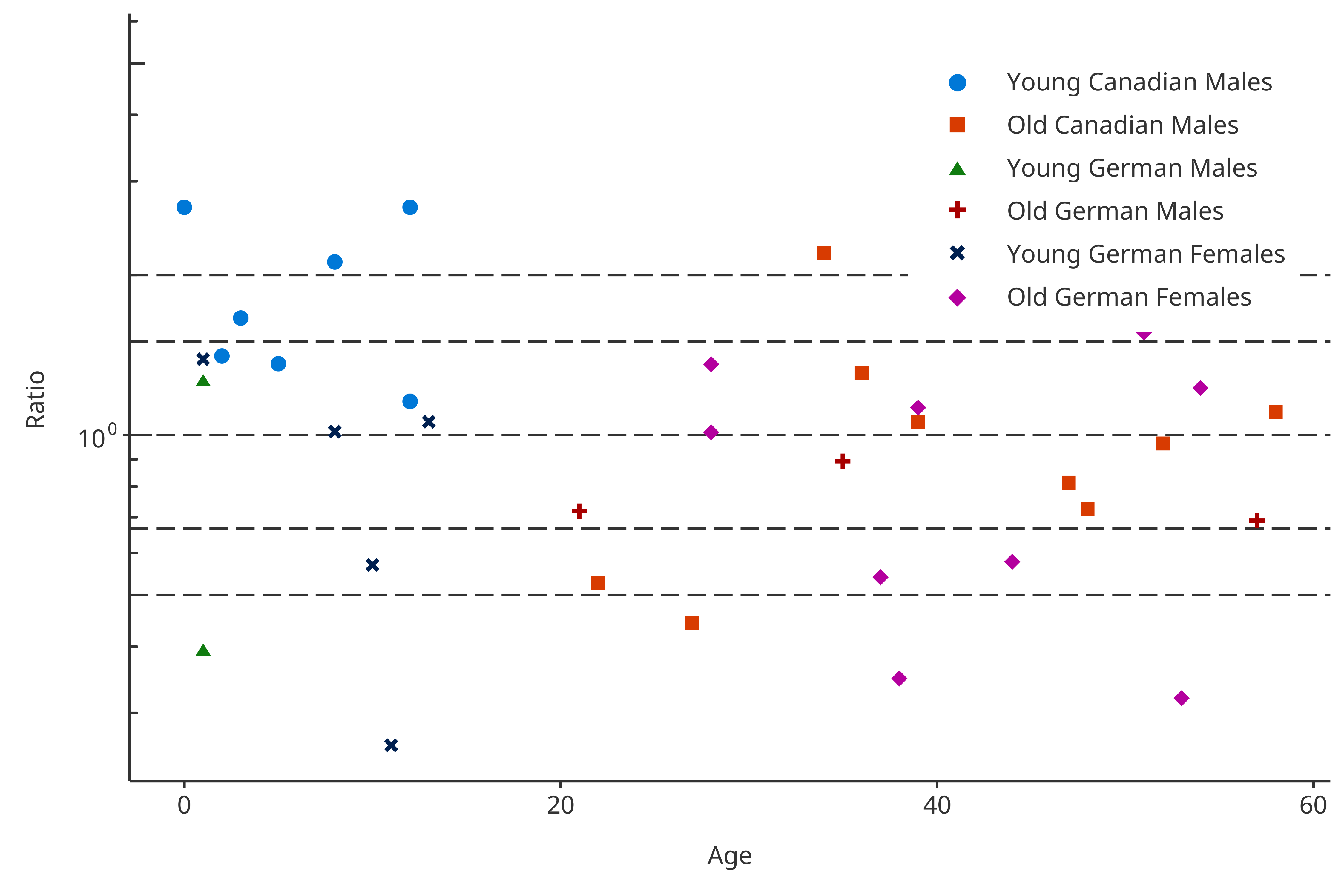
The last examples uses another feature available in the
groupMapping class. The class can be initialized using a
data.frame where the last column of the data.frame will be
used to split the data. In the following example, the data.frame is the
following:
| AgeBin | Country | Sex | Group |
|---|---|---|---|
| Peds | Canada | Male | Young Canadian Males |
| Adults | Canada | Male | Old Canadian Males |
| Peds | Germany | Male | Young German Males |
| Adults | Germany | Male | Old German Males |
| Peds | France | Male | Young French Males |
| Adults | France | Male | Old French Males |
| Peds | Canada | Female | Young Canadian Females |
| Adults | Canada | Female | Old Canadian Females |
| Peds | Germany | Female | Young German Females |
| Adults | Germany | Female | Old German Females |
| Peds | France | Female | Young French Females |
| Adults | France | Female | Old French Females |
The dataMapping introduced below will split the
color and shape using the data frame.
dataMappingDF <- PKRatioDataMapping$new(
  x = "Age",
  y = "Ratio",
  color = groupDataFrame,
  shape = groupDataFrame
)
plotPKRatio(
  data = pkRatioData[!(pkRatioData$Country %in% "France"), ],
  dataMapping = dataMappingDF
)
2.4.2 PK values defined in lines
In PK ratio examples, usually horizontal lines are added allowing to
flag values in and out of the [0.67-1.5] as well as [0.5-2.0] ranges.
The value mapping these horizontal lines was predefined as a list:
“pkRatioLine1” is 1, “pkRatioLine2” is c(0.67, 1.5) and “pkRatioLine3”
is c(0.5, 2). Consequently, for any default
PKRatioDataMapping, you have:
linesMapping <- PKRatioDataMapping$new()
linesMapping$lines
#> $pkRatio1
#> [1] 1
#>
#> $pkRatio2
#> [1] 1.5000000 0.6666667
#>
#> $pkRatio3
#> [1] 2.0 0.5
Overwriting these value is possible by updating the value either when initializing the mapping or afterwards. For instance:
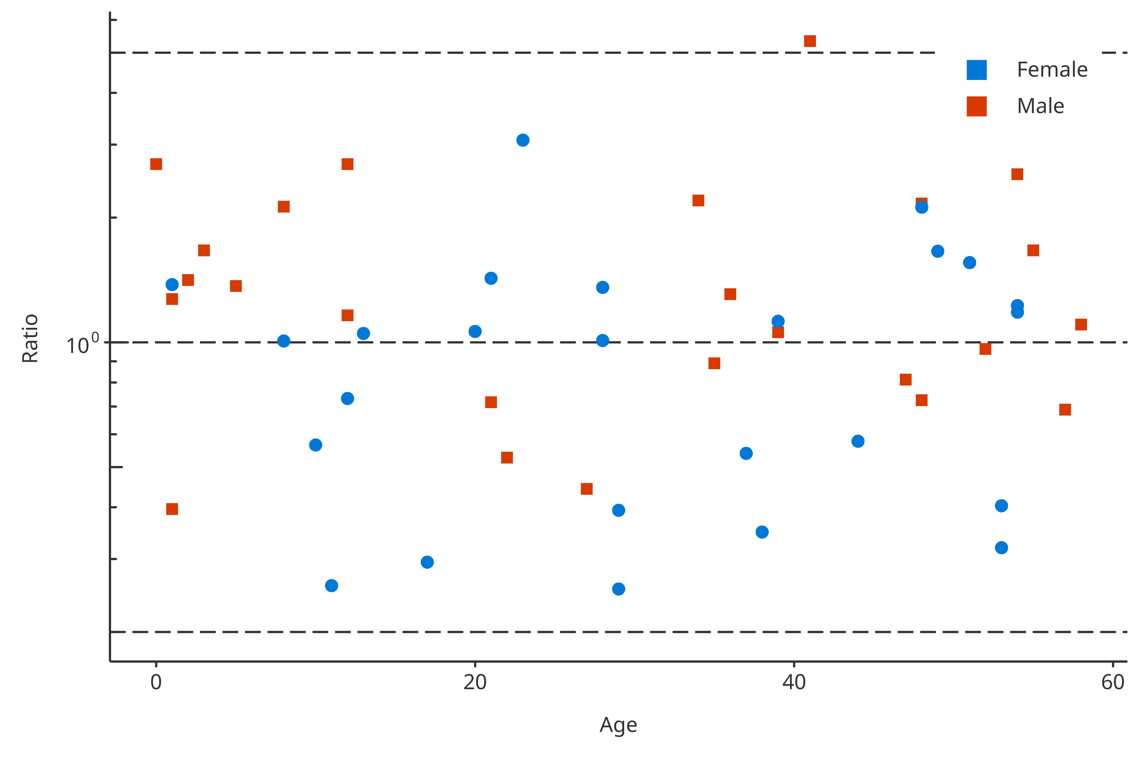
linesMapping <- PKRatioDataMapping$new(
  lines = list(pkRatio1 = 1, pkRatio2 = c(0.2, 5)),
  x = "Age",
  y = "Ratio",
  color = "Sex"
)
plotPKRatio(
  data = pkRatioData,
  dataMapping = linesMapping
)
2.5. Qualification of PK Ratios
The qualification of the PK Ratios can be performed using
getPKRatioMeasure. This function return a
data.frame with the PK ratios within specific ranges. As a
default, these ranges are within 1.5 and 2 folds. However, they can be
updated using the option ratioLimits = when running the
function.
# Test of getPKRatioMeasure
PKRatioMeasure <- getPKRatioMeasure(data = pkRatioData[, c("Age", "Ratio")])

knitr::kable(
  x = PKRatioMeasure,
  caption = "Qualification of PK Ratios"
)| Number | Ratio | |
|---|---|---|
| Points Total | 50 | NA |
| Points within 1.5-fold | 24 | 0.48 |
| Points within 2-fold | 32 | 0.64 |
2.6. Plot Configuration
To configure the plot properties,
PKRatioPlotConfiguration objects can be used. They combine
multiple features that set the plot properties. PK ratio plot consists
in lines and points. As illustrated in the vignette
related to PlotConfiguration objects and Theme, you
can tune the aesthetic maps and their selections (see
vignette("plot-configuration") and
vignette("theme-maker")). Colors, shapes and size of the PK
ratio scatter points can be tuned in the plotConfiguration
points field. Likewise, colors, linetype and size of the PK
ratio lines can be tuned in the plotConfiguration lines
field.