require(tlf)
#> Loading required package: tlf
# Place default legend position above the plot for prettier time profile plots
setDefaultLegendPosition(LegendPositions$outsideTop)
1. Introduction
The following vignette aims at documenting and illustrating workflows
for producing Time Profile plots using the tlf-Library.
Time profile plots aims at comparing observed and simulated data along time. In such plots, observed data are usually plotted as scatter points with errorbars showing population range or confidence intervals; while simulated data are usually plotted using lines with shaded ribbons showing population range or confidence intervals.
2. Definition of the time profile functions and classes
2.1. plotTimeProfile
Besides, the usual tlf input arguments commonly used by
the plot functions (data, metaData,
dataMapping, plotConfiguration and
plotObject), the function plotTimeProfile also
includes the following optional input arguments:
-
observedData: A data.frame to use for plot. Unlikedata, meant for simulated data, plotted as lines and ribbons;observedDatais plotted as scatter points and errorbars. -
observedDataMapping: AnObservedDataMappingobject mappingx,y,ymin,ymax, and aesthetic groups to their variable names ofobservedData.
2.2. Data Mappings
2.2.1. dataMapping argument
For time profile simulated data, TimeProfileDataMapping
objects are required through the dataMapping argument of
the function plotTimeProfile.
As highlighted below, the class is initialized using the method
$new. The optional arguments ymin and
ymax define the shaded area of population range or
confidence interval. The argument y is optional,
only if ymin and ymax are
provided.
It can be noted that the argument group can be used to
group the data by these aesthetics.
TimeProfileDataMapping$new(
x,
y = NULL,
ymin = NULL,
ymax = NULL,
group = NULL
)
2.2.2. observedDataMapping argument
For time profile observed data, ObservedDataMapping
objects are required through the observedDataMapping
argument of the function plotTimeProfile.
As highlighted below, the class is initialized using the method
$new. The optional arguments ymin and
ymax define the error bars of population range or
confidence interval. The optional argument error can be
used instead to calculate the errorbars from the variable
y.
The argument mdv, meant for missing dependent variable,
is a flag inspired from Nonmem for excluding data from the final time
profile plot.
It can be noted that the argument group can be used to
group the data by these aesthetics.
ObservedDataMapping$new(
x,
y,
error = NULL,
ymin = NULL,
ymax = NULL,
group = NULL,
mdv = NULL
)
2.2.3. Remaining TODOs
Some time profiles can also show another quantity in parallel and
whose unit is different. A right axis is usually added for such plots to
describe the values of that quantity. The
TimeProfileDataMapping and ObservedData
objects do not support yet a y2 argument for displaying
data on the right axis.
3. Examples
For the examples presented in the sequel, two simulated and two observed datasets are created below:
# Simulation time
simTime <- seq(0, 24, 0.1)

# metaData will be used during the smart mapping
# to label the axes as "dimension [unit]"
metaData <- list(
  time = list(
    dimension = "Time",
    unit = "h"
  ),
  concentration = list(
    dimension = "Concentration",
    unit = "mg/l"
  )
)
# Spread metaData to min/max
metaData$maxConcentration <- metaData$concentration
metaData$minConcentration <- metaData$concentration

# Simulated data 1: exponential decay
simData1 <- data.frame(
  time = simTime,
  concentration = 15 * exp(-0.1 * simTime),
  minConcentration = 12 * exp(-0.12 * simTime),
  maxConcentration = 18 * exp(-0.08 * simTime),
  caption = "Simulated Data 1"
)

# Simulated data 2: first order absorption with exponential decay
simData2 <- data.frame(
  time = simTime,
  concentration = 10 * exp(-0.1 * simTime) * (1 - exp(-simTime)),
  minConcentration = 8 * exp(-0.12 * simTime) * (1 - exp(-simTime)),
  maxConcentration = 12 * exp(-0.08 * simTime) * (1 - exp(-simTime)),
  caption = "Simulated Data 2"
)
# Observed data 1
obsData1 <- data.frame(
  time = c(1, 3, 6, 12, 24),
  concentration = c(11.7, 8.4, 7.5, 3.6, 1.0),
  sd = c(0.204, 0.21, 0.241, 0, 0.18),
  caption = "Observed Data 1"
)

# Observed data 2
obsData2 <- data.frame(
  time = c(0, 1, 3, 6, 12, 24),
  concentration = c(0, 6.1, 7.3, 4.4, 3.2, 1.1),
  minConcentration = c(0, 5.7, 7.0, 4.3, 2.5, 0.8),
  maxConcentration = c(0, 7.1, 8.2, 5.8, 3.3, 1.11),
  caption = "Observed Data 2"
)
The following sections show how to plot a Time Profile for specific scenarios
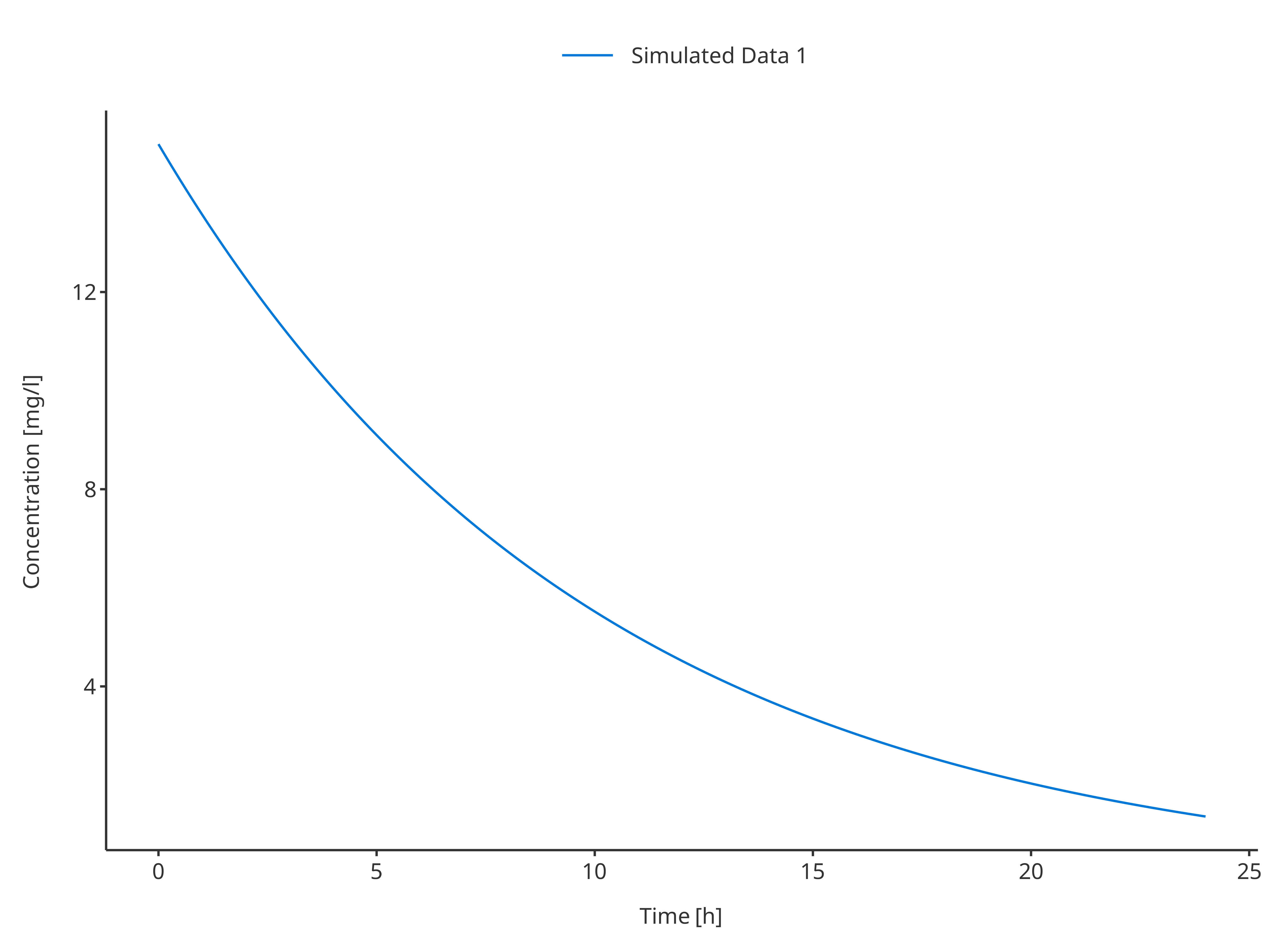
3.1. Plot simulated data only
3.1.1 Single simulation
# Define Data Mapping
simDataMapping <- TimeProfileDataMapping$new(
  x = "time",
  y = "concentration",
  group = "caption"
)

plotTimeProfile(
  data = simData1,
  metaData = metaData,
  dataMapping = simDataMapping
)
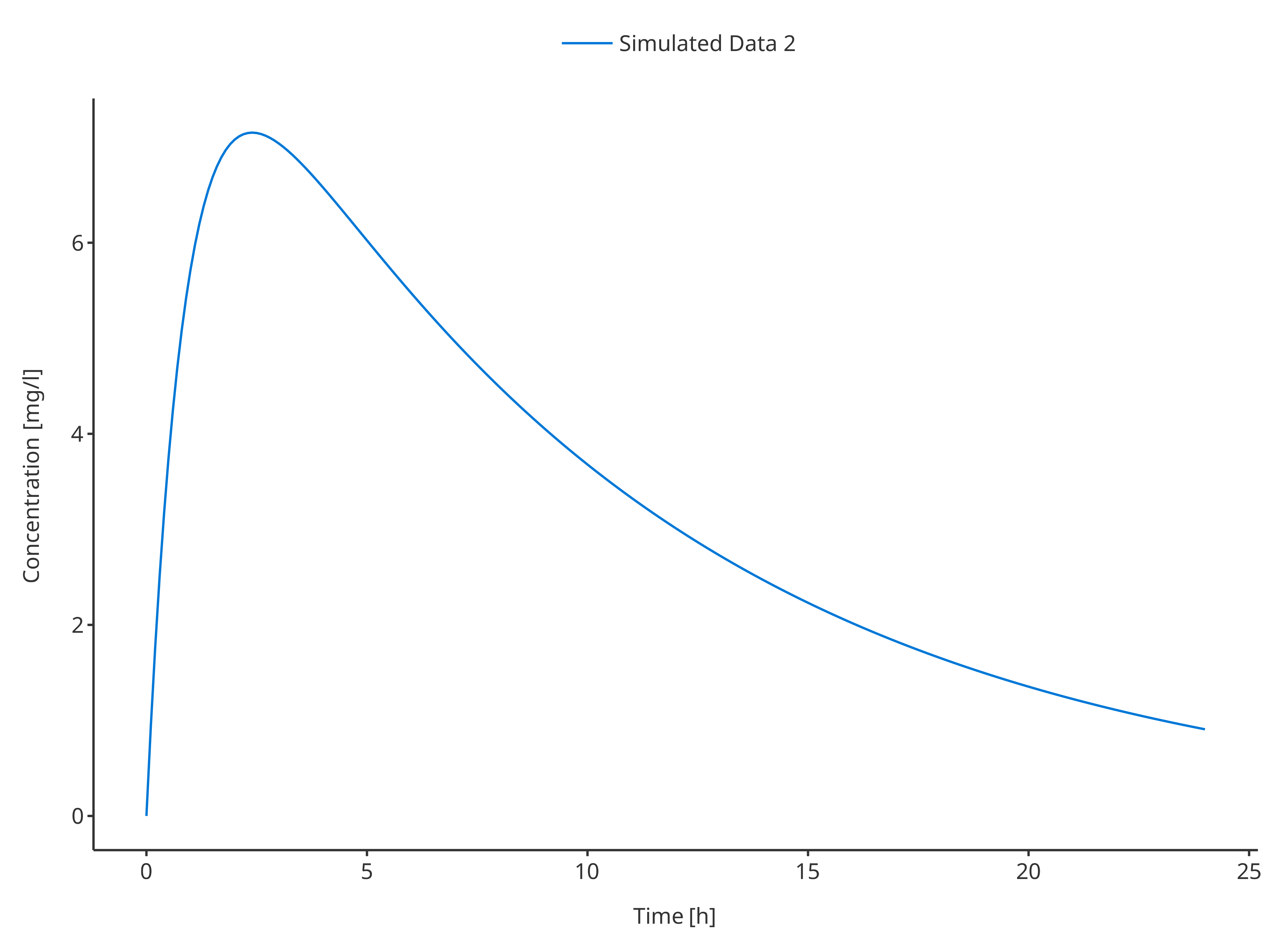
plotTimeProfile(
  data = simData2,
  metaData = metaData,
  dataMapping = simDataMapping
)
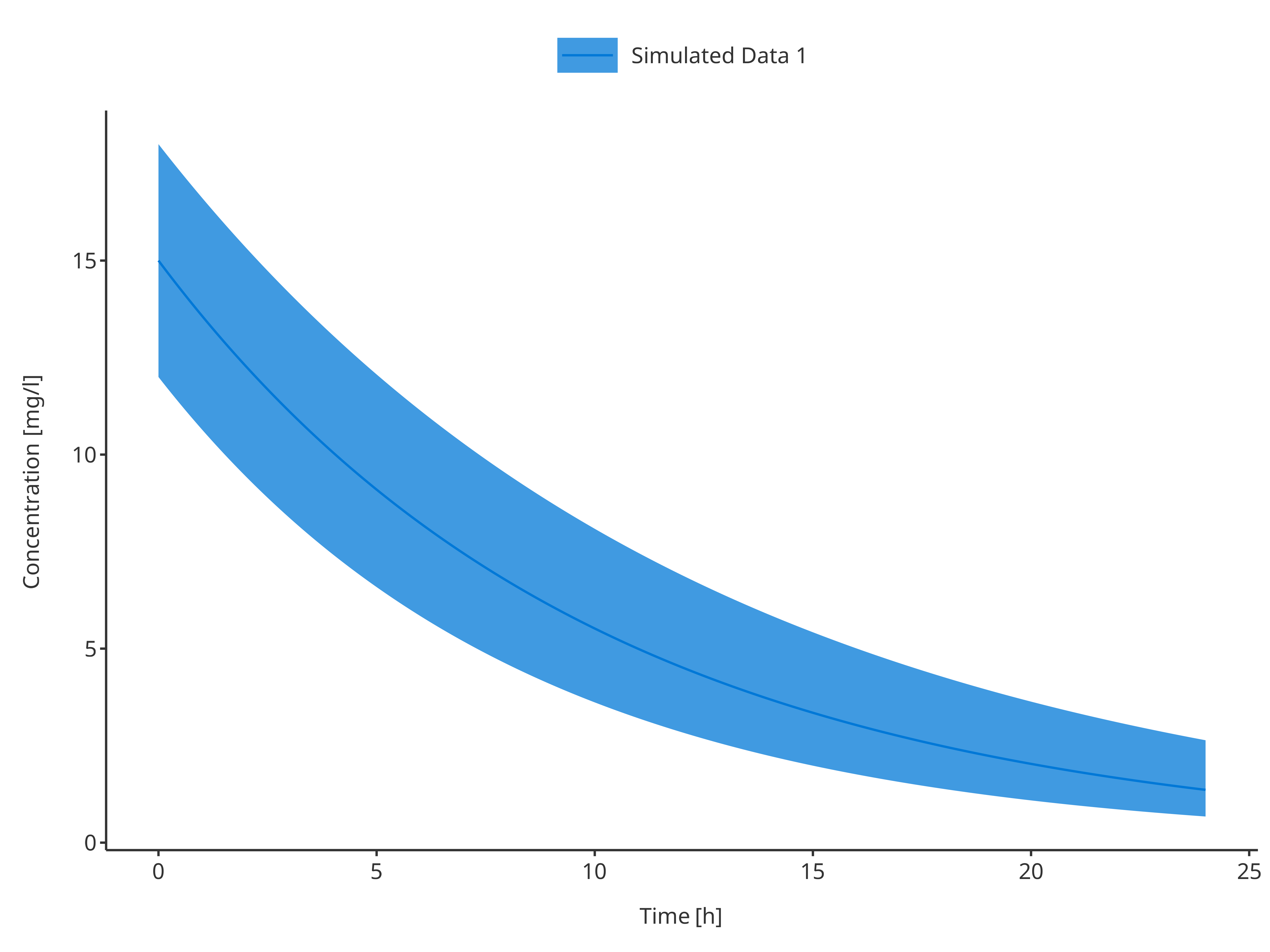
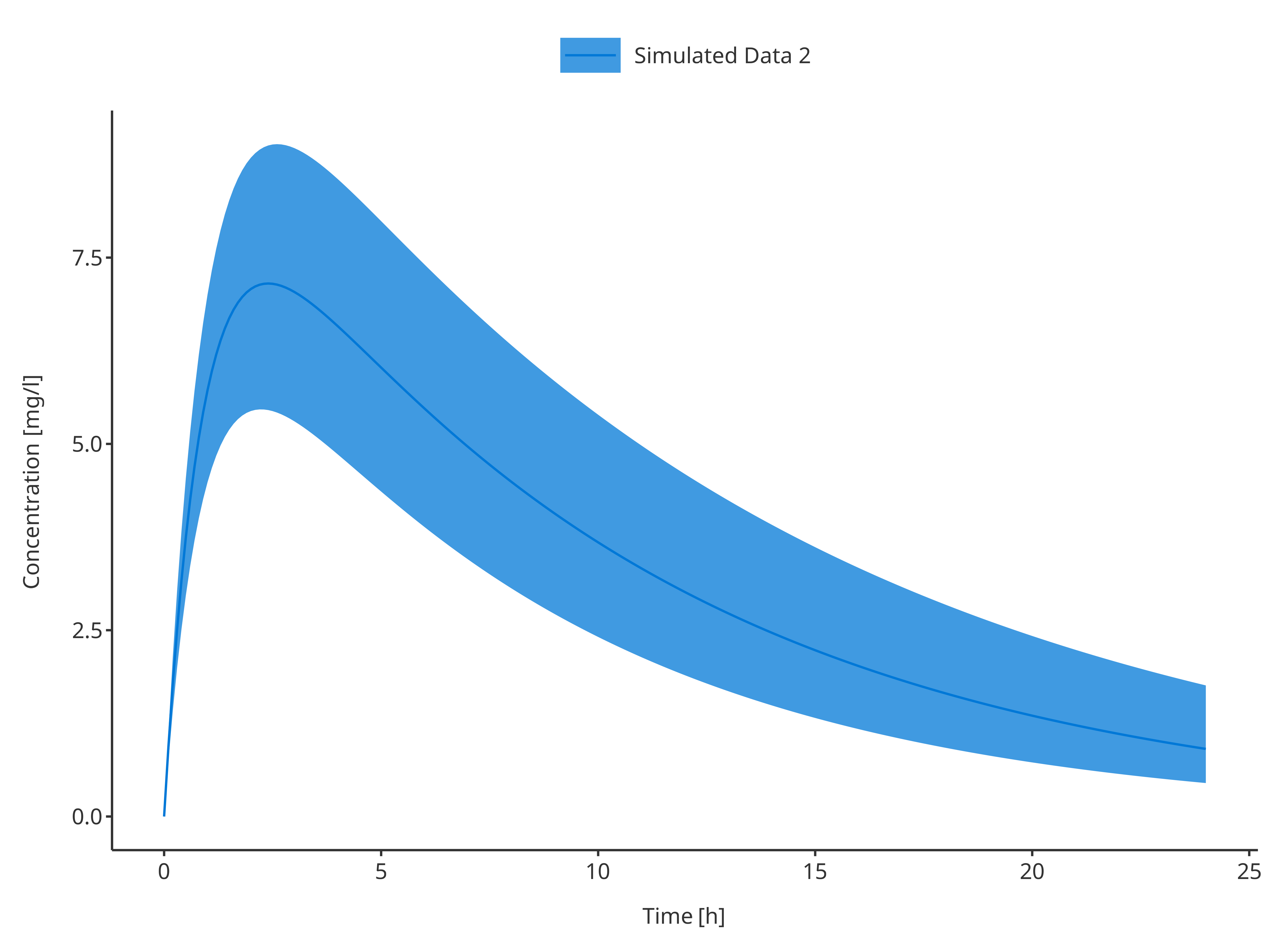
3.1.2. Single simulation with confidence interval
# Define Data Mapping
simDataMapping <- TimeProfileDataMapping$new(
  x = "time",
  y = "concentration",
  ymin = "minConcentration",
  ymax = "maxConcentration",
  group = "caption"
)

plotTimeProfile(
  data = simData1,
  metaData = metaData,
  dataMapping = simDataMapping
)
plotTimeProfile(
  data = simData2,
  metaData = metaData,
  dataMapping = simDataMapping
)
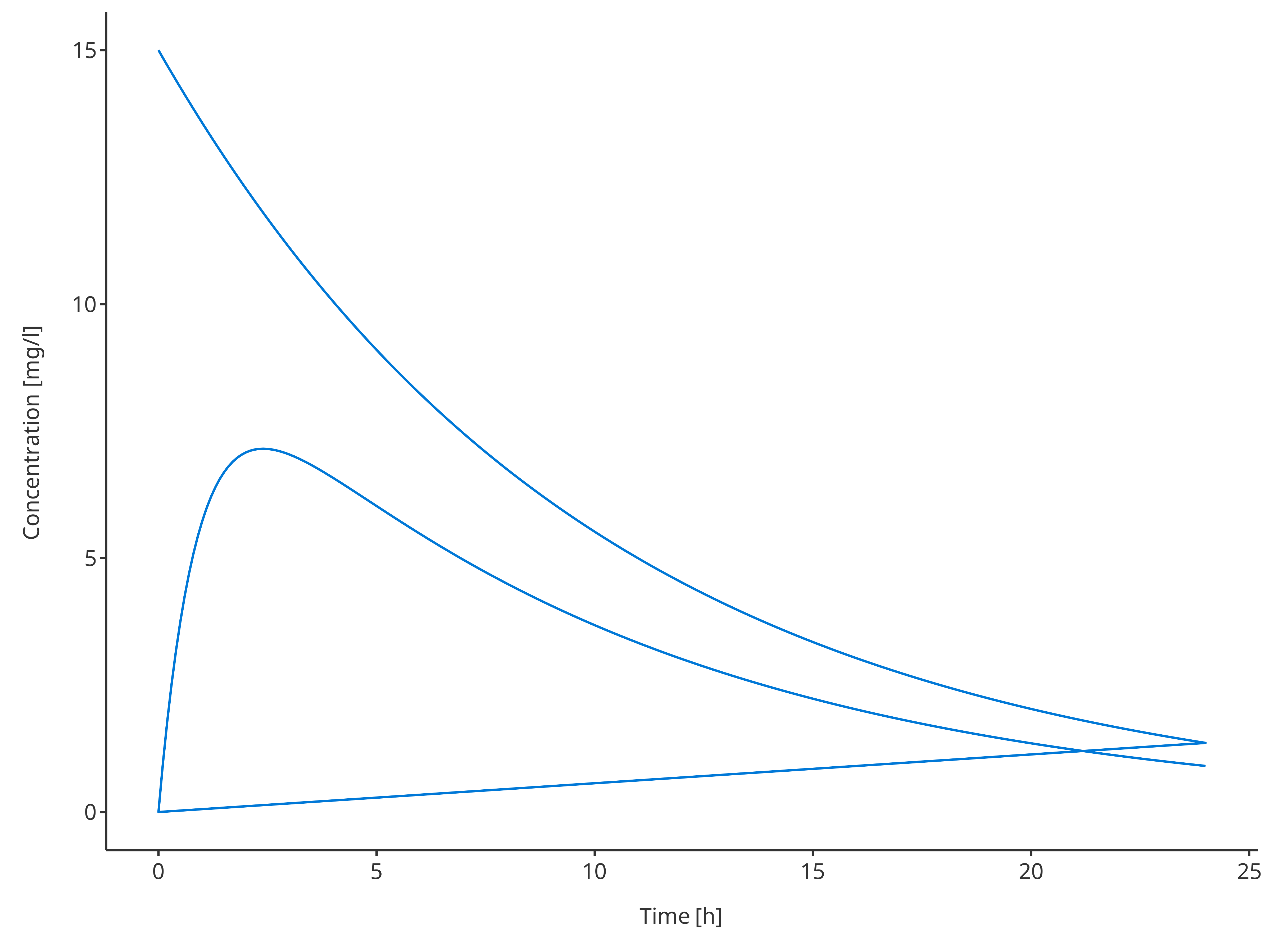
3.1.3. Multiple simulations
# Define Data Mapping
# Not using a group here will plot both profiles
# but as they were the same data
simDataMapping <- TimeProfileDataMapping$new(
  x = "time",
  y = "concentration"
)

plotTimeProfile(
  data = rbind.data.frame(
    simData1,
    simData2
  ),
  metaData = metaData,
  dataMapping = simDataMapping
)
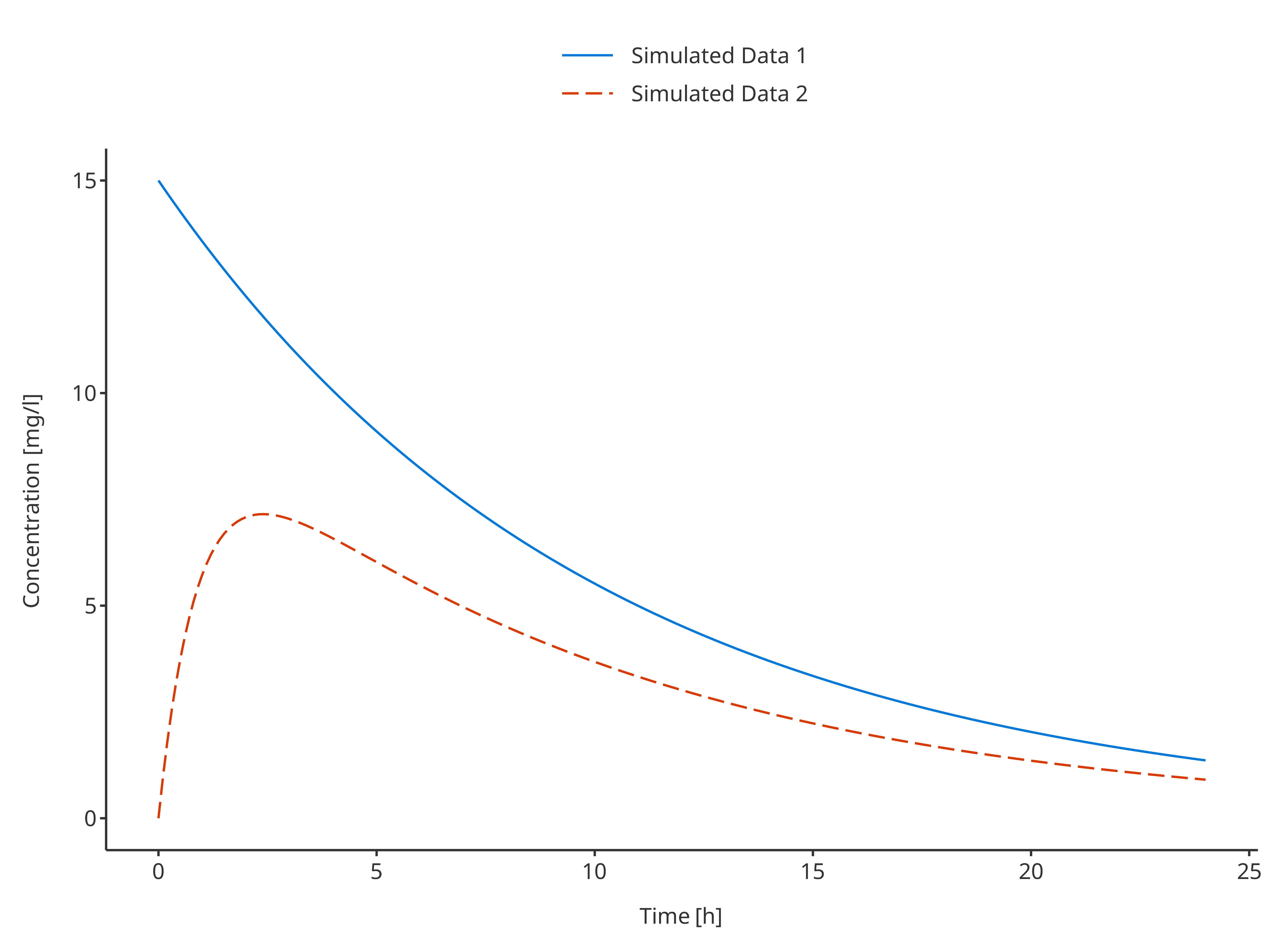
# Define Data Mapping
# Using a group to plot both profiles

simDataMapping <- TimeProfileDataMapping$new(
  x = "time",
  y = "concentration",
  group = "caption"
)

plotTimeProfile(
  data = rbind.data.frame(
    simData1,
    simData2
  ),
  metaData = metaData,
  dataMapping = simDataMapping
)
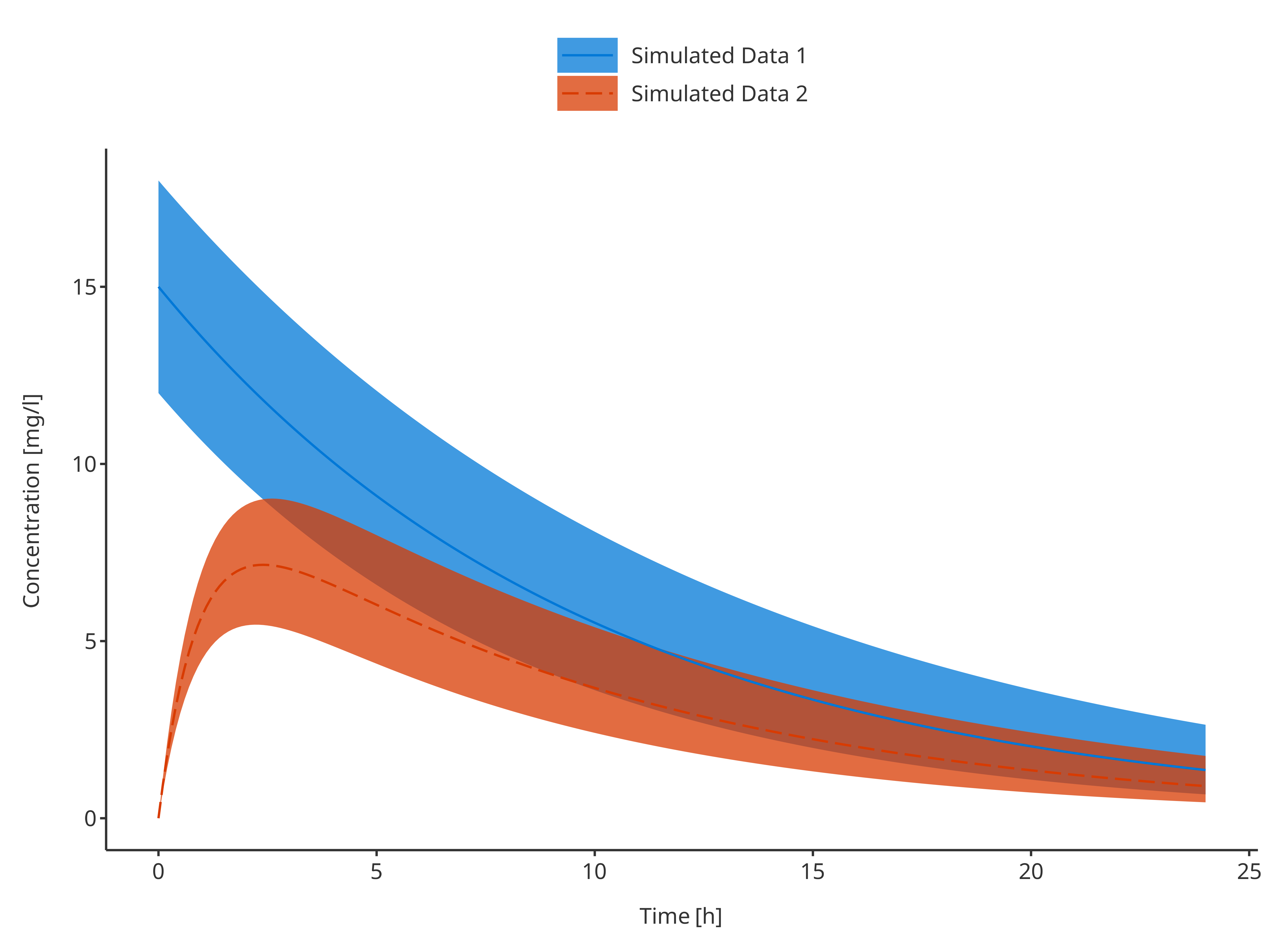
3.1.4. Multiple simulations with confidence interval
# Define Data Mapping
# ymin and ymax define the CI
simDataMapping <- TimeProfileDataMapping$new(
  x = "time",
  y = "concentration",
  ymin = "minConcentration",
  ymax = "maxConcentration",
  group = "caption"
)

plotTimeProfile(
  data = rbind.data.frame(
    simData1,
    simData2
  ),
  metaData = metaData,
  dataMapping = simDataMapping
)
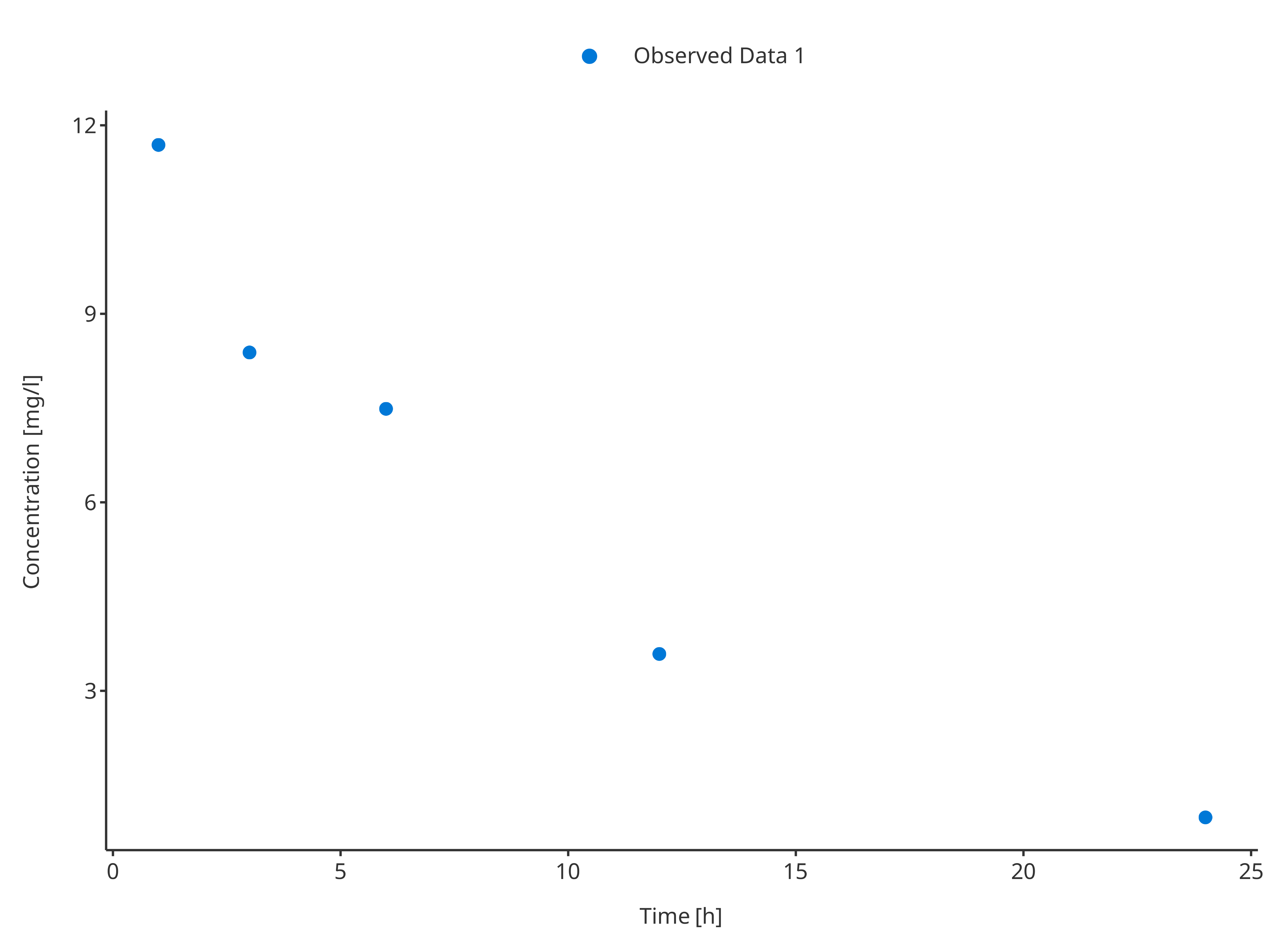
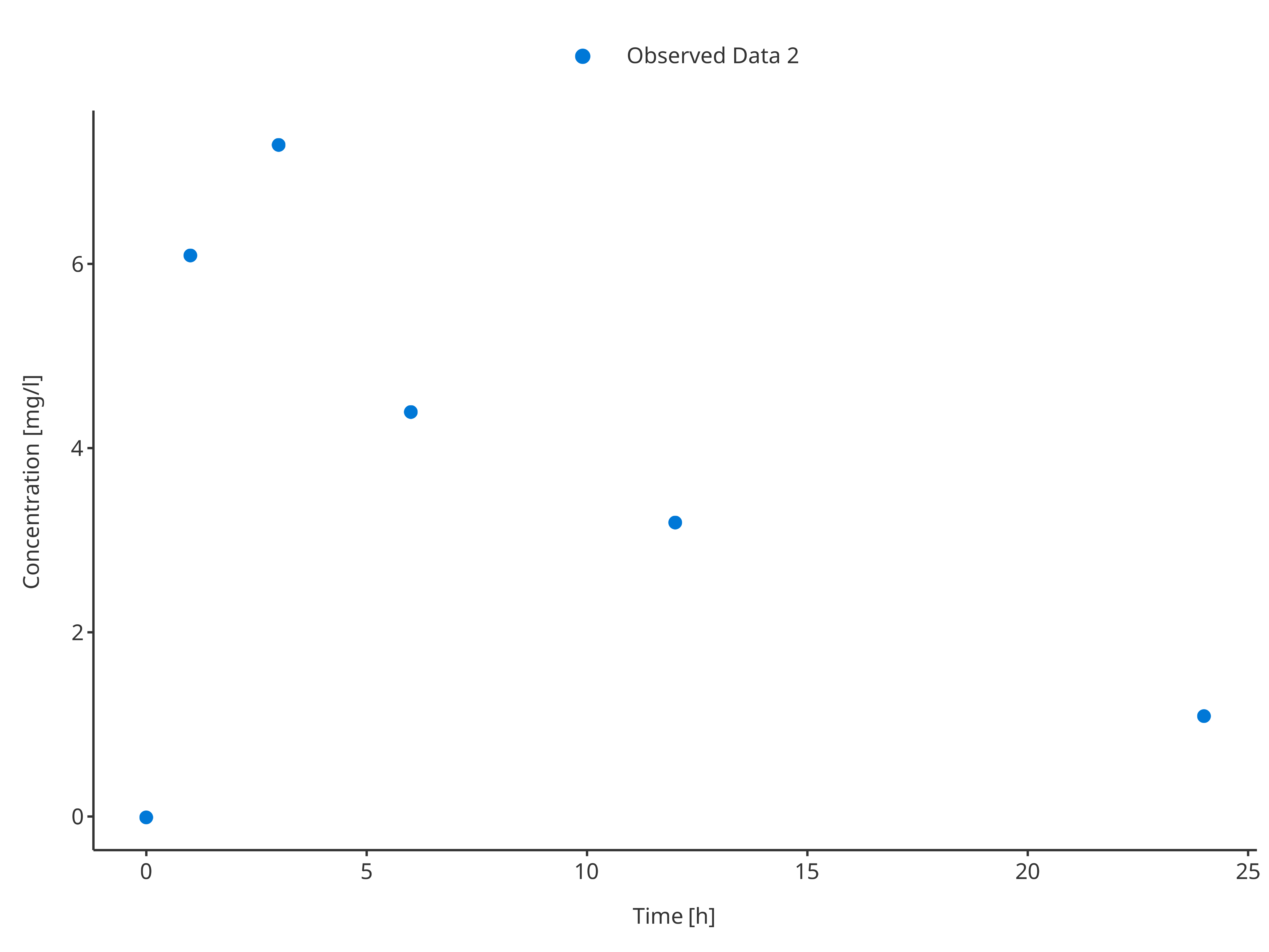
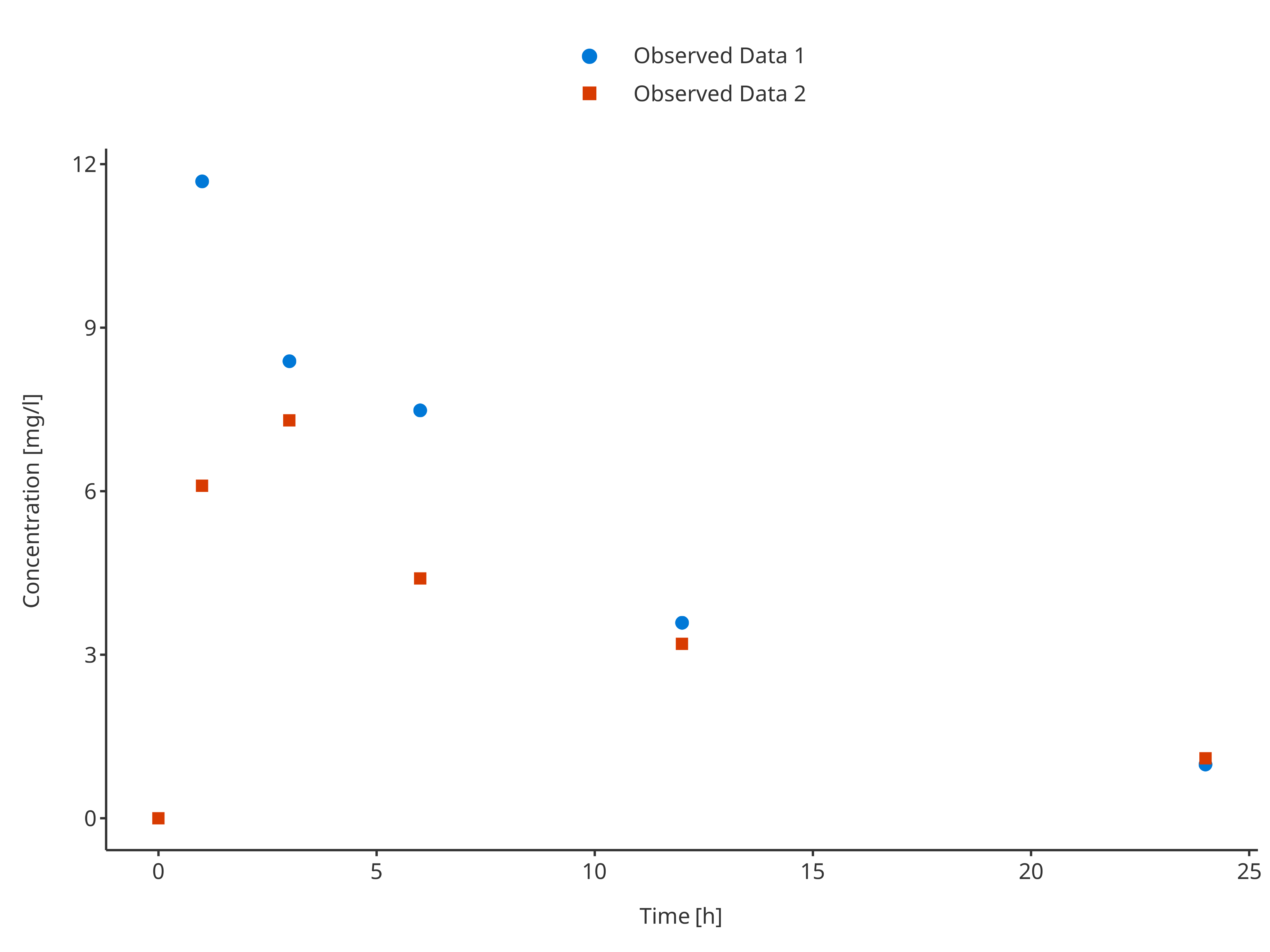
3.2. Plot observed data only
3.2.1. Single observed data set
# Define Data Mapping
obsDataMapping <- ObservedDataMapping$new(
  x = "time",
  y = "concentration",
  group = "caption"
)

plotTimeProfile(
  observedData = obsData1,
  metaData = metaData,
  observedDataMapping = obsDataMapping
)
plotTimeProfile(
  observedData = obsData2,
  metaData = metaData,
  observedDataMapping = obsDataMapping
)
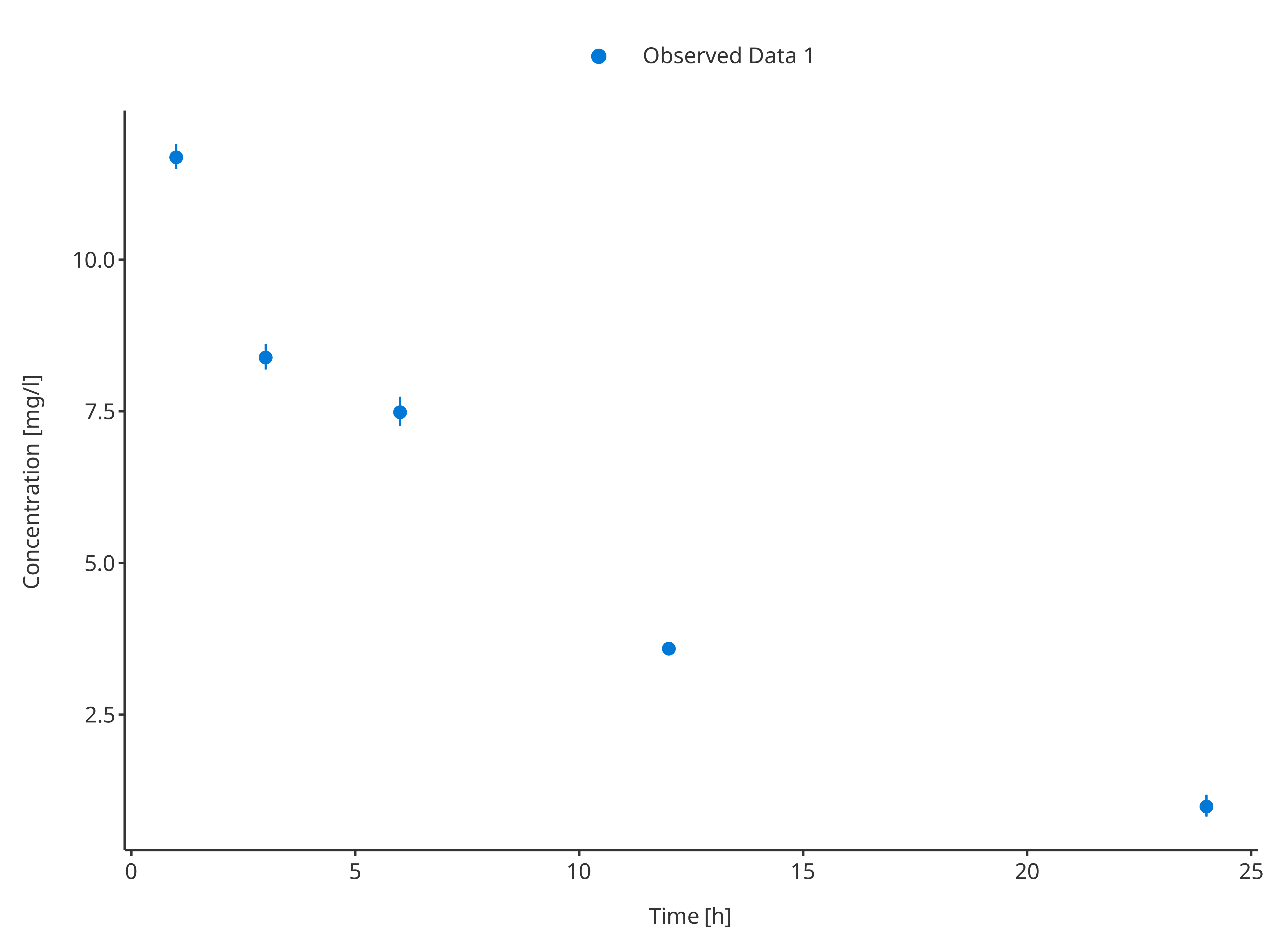
3.2.2. Single simulation with confidence interval
For the first dataset, the uncertainty/error was defined as standard
deviation using the variable "sd". This variable will be
used by the ObservedDataMapping object to create
corresponding ymin and ymax values for the
error bars.
Tips
- For data that include errorbars only partially,
NAvalues cannot be used and should be replaced by0for error variable oryforyminandymaxvariables. - For logarithmic plots, negative
yminvalues of errorbars should be replaced byybeforehand in order to still see theymaxrange of the errorbars.
# Define Data Mapping
obsDataMapping1 <- ObservedDataMapping$new(
  x = "time",
  y = "concentration",
  error = "sd",
  group = "caption"
)

plotTimeProfile(
  observedData = obsData1,
  metaData = metaData,
  observedDataMapping = obsDataMapping1
)
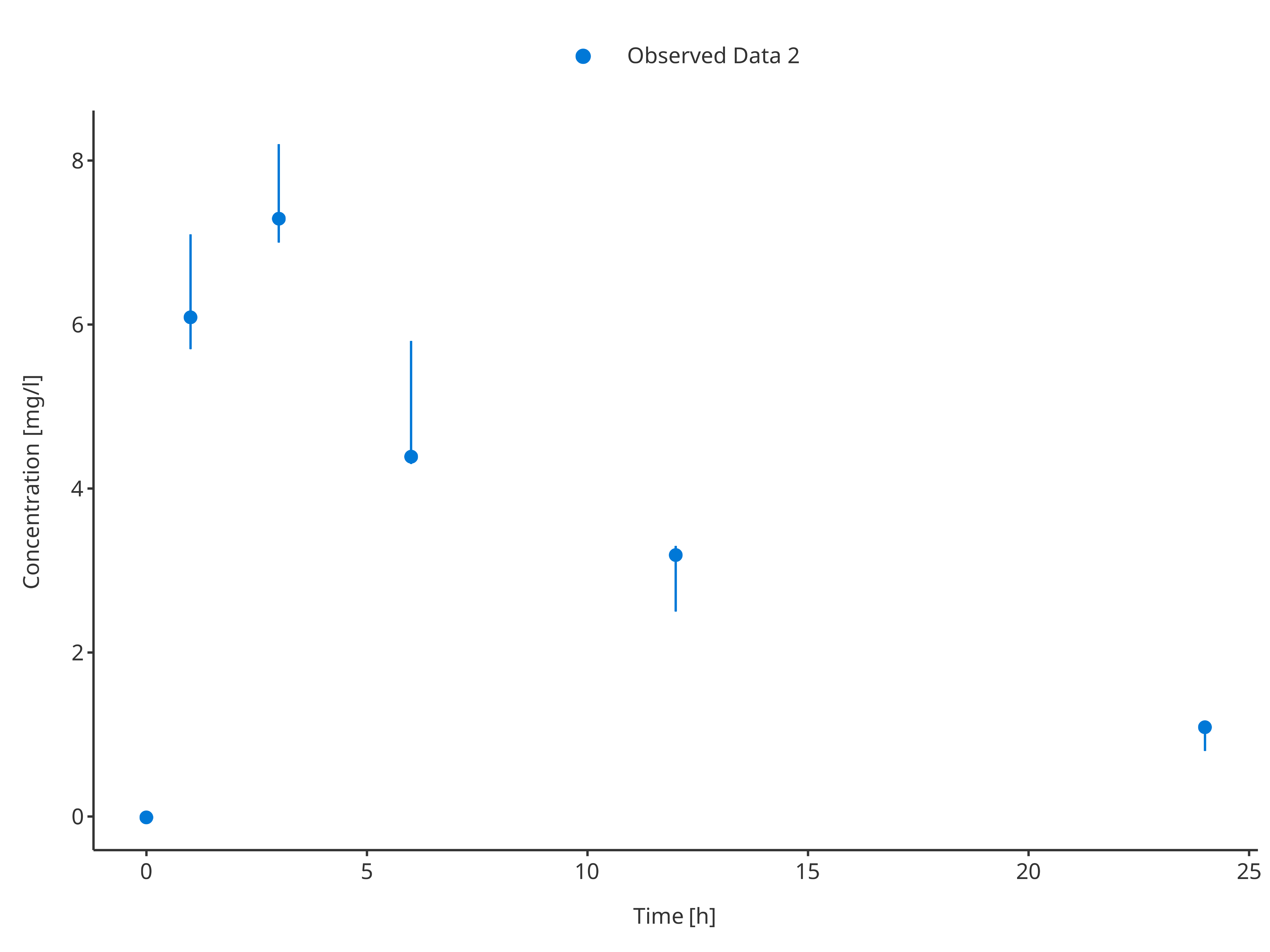
For the second dataset, the uncertainty/error was defined as
"minConcentration" and "minConcentration",
they are input directly as ymin and ymax and
will be taken as is by the ObservedDataMapping object.
# Define Data Mapping
obsDataMapping2 <- ObservedDataMapping$new(
  x = "time",
  y = "concentration",
  ymin = "minConcentration",
  ymax = "maxConcentration",
  group = "caption"
)

plotTimeProfile(
  observedData = obsData2,
  metaData = metaData,
  observedDataMapping = obsDataMapping2
)
3.2.3. Multiple observed data sets
# Define Data Mapping
obsDataMapping <- ObservedDataMapping$new(
  x = "time",
  y = "concentration",
  group = "caption"
)

plotTimeProfile(
  observedData = rbind.data.frame(
    obsData1[, c("time", "concentration", "caption")],
    obsData2[, c("time", "concentration", "caption")]
  ),
  metaData = metaData,
  observedDataMapping = obsDataMapping
)
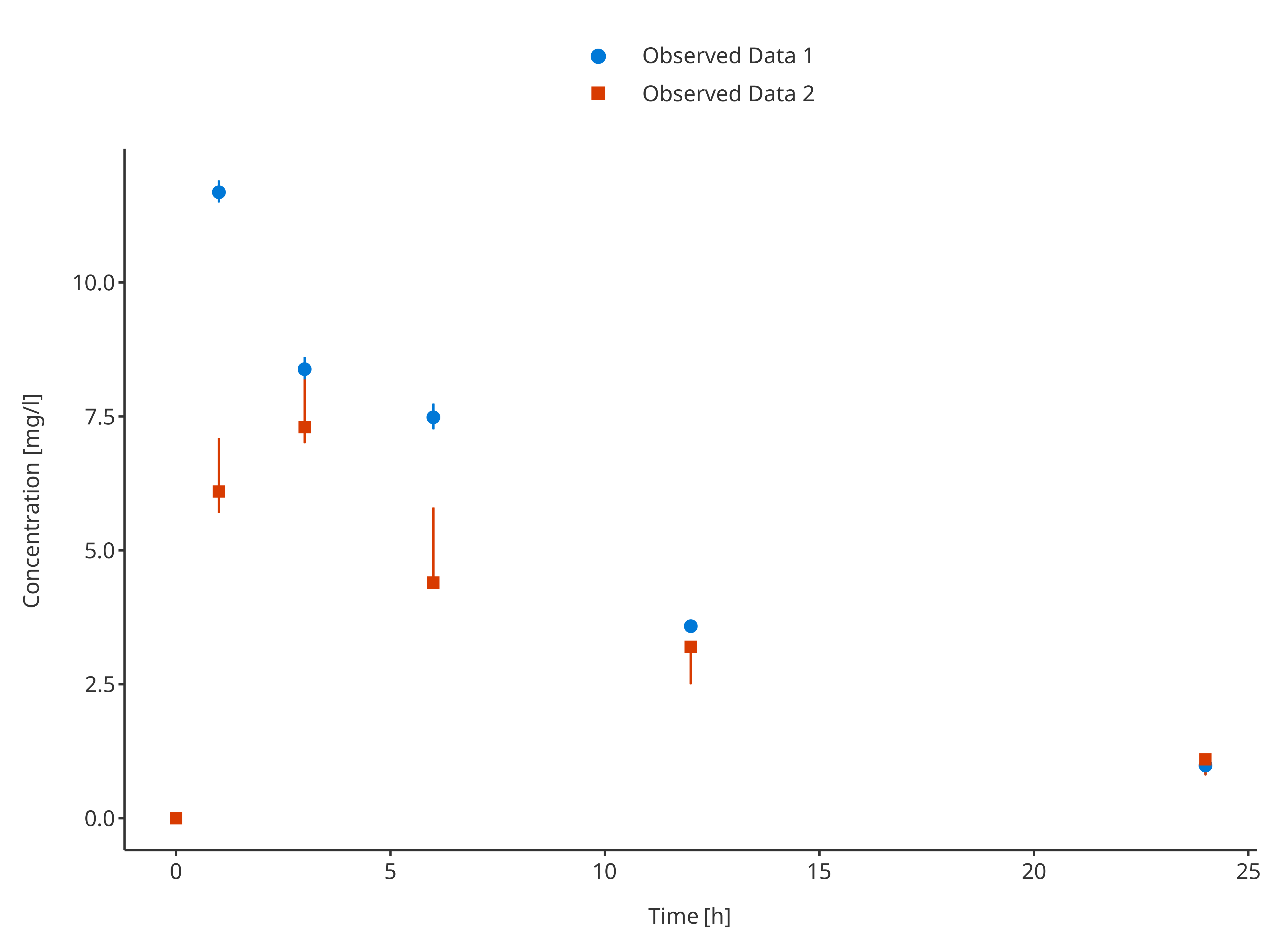
3.2.4. Multiple observed data sets with confidence interval
In this example, the observed data were not using the same way of displaying errors. Before plotting, the data needs to be merged in a consistent way to let the dataMapping know which variable(s) to use.
Below, ymin and ymax were consequently
calculated for obsData1 before merging.
# Use common variable before usinf rbind.data.frame
obsData1$minConcentration <- obsData1$concentration - obsData1$sd
obsData1$maxConcentration <- obsData1$concentration + obsData1$sd
obsData2$sd <- 0

# Define Data Mapping
obsDataMapping <- ObservedDataMapping$new(
  x = "time",
  y = "concentration",
  ymin = "minConcentration",
  ymax = "maxConcentration",
  group = "caption"
)

plotTimeProfile(
  observedData = rbind.data.frame(
    obsData1,
    obsData2
  ),
  metaData = metaData,
  observedDataMapping = obsDataMapping
)
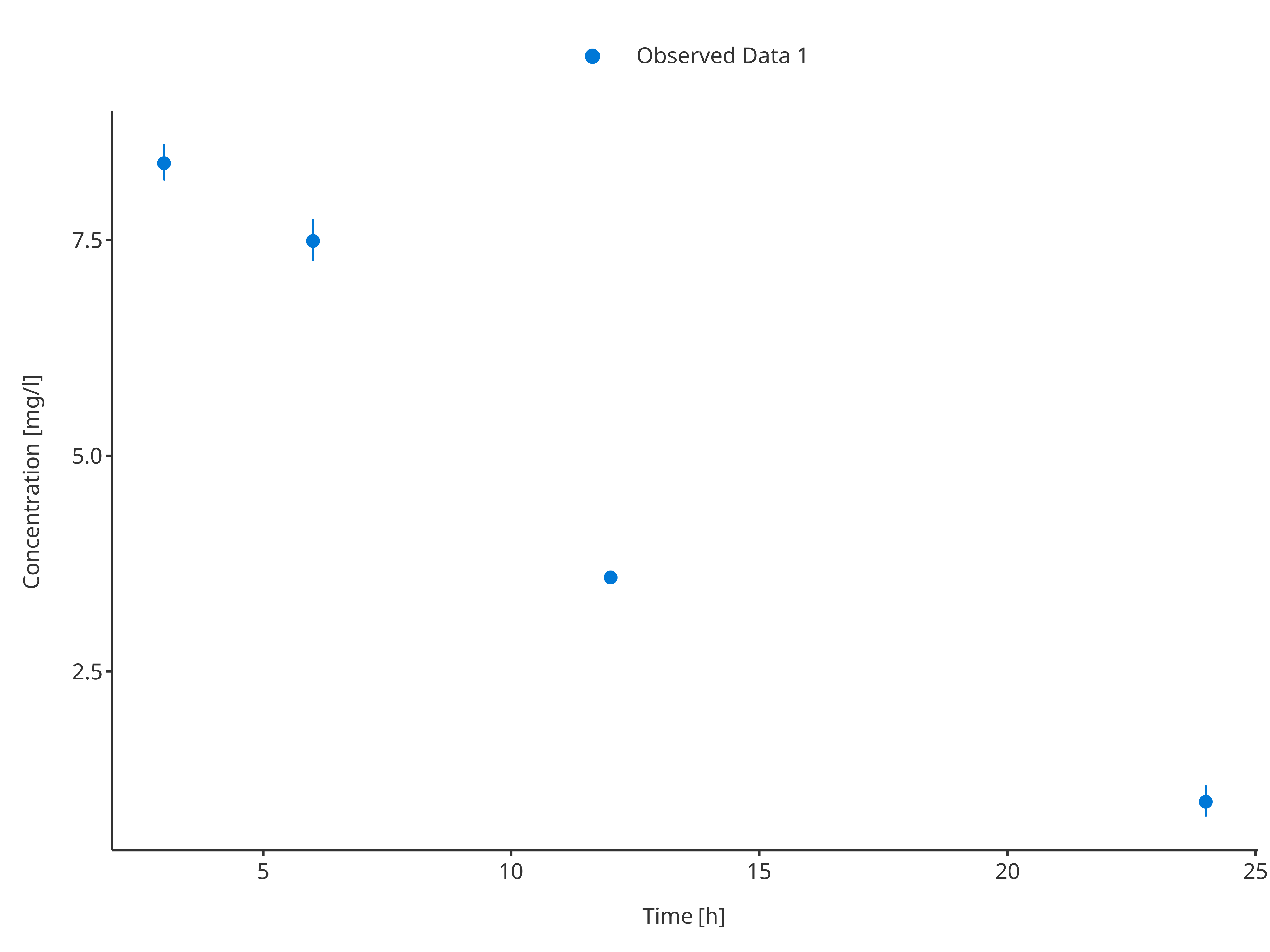
3.2.4. Missing Dependent Variable (mdv)
The following code flags all values higher than 10 as
mdv, leading to a plot without any observed data points
higher than 10 (removing the first observation)
# Use common variable before usinf rbind.data.frame
mdvData <- obsData1
mdvData$mdv <- mdvData$concentration > 10

# Define Data Mapping
obsDataMapping <- ObservedDataMapping$new(
  x = "time",
  y = "concentration",
  ymin = "minConcentration",
  ymax = "maxConcentration",
  group = "caption",
  mdv = "mdv"
)

plotTimeProfile(
  observedData = mdvData,
  metaData = metaData,
  observedDataMapping = obsDataMapping
)
3.3. Plot simulated and observed data
By combining data and their dataMapping
with observedData and their
observedDataMapping, complex time profiles comparing
observed and simulated data can be plotted.
3.3.1. Single simulation and observed data set
# Define Data Mappings
simDataMapping <- TimeProfileDataMapping$new(
  x = "time",
  y = "concentration",
  group = "caption"
)

obsDataMapping <- ObservedDataMapping$new(
  x = "time",
  y = "concentration",
  group = "caption"
)

plotTimeProfile(
  data = simData1,
  observedData = obsData1,
  metaData = metaData,
  dataMapping = simDataMapping,
  observedDataMapping = obsDataMapping
)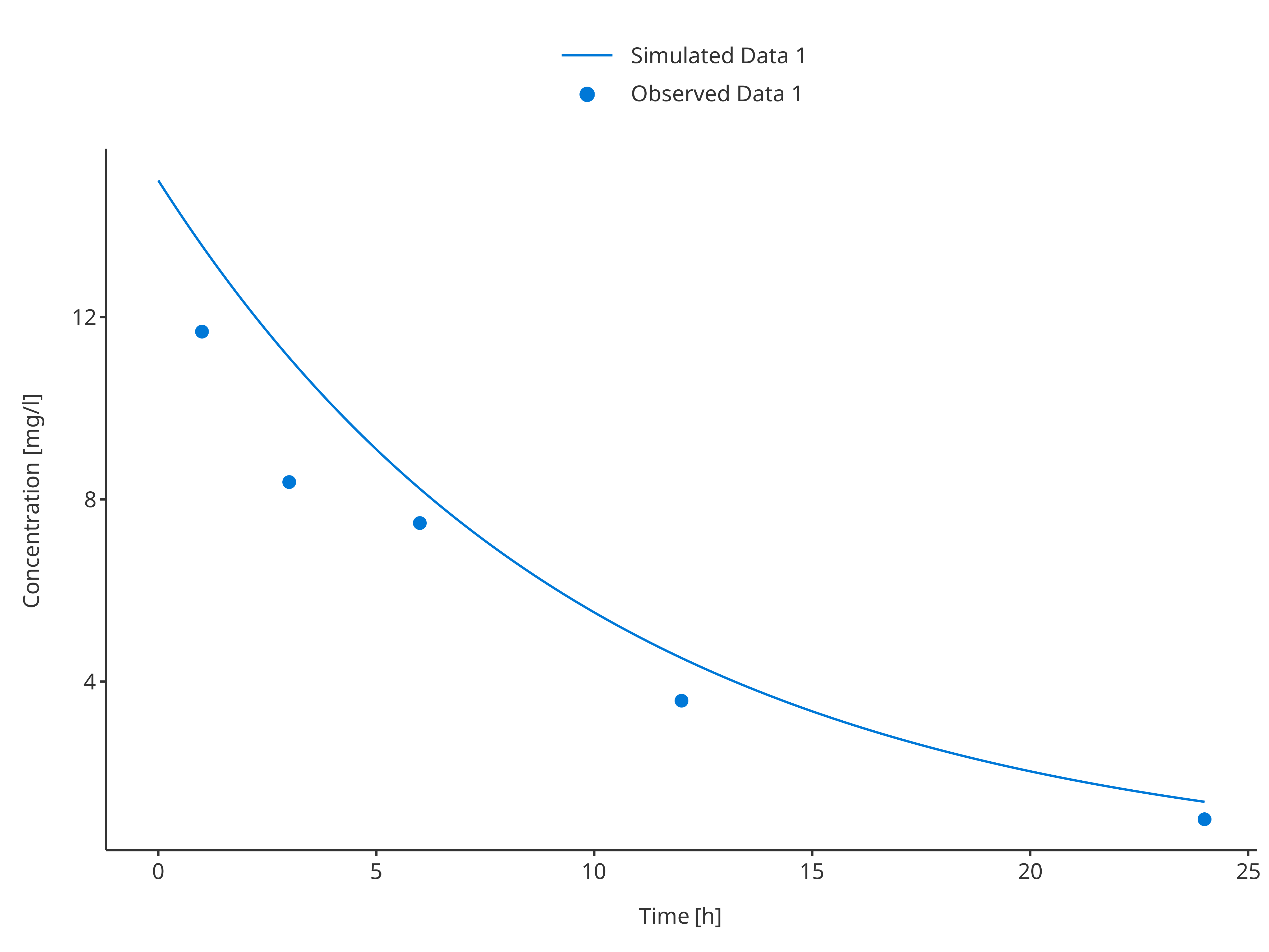
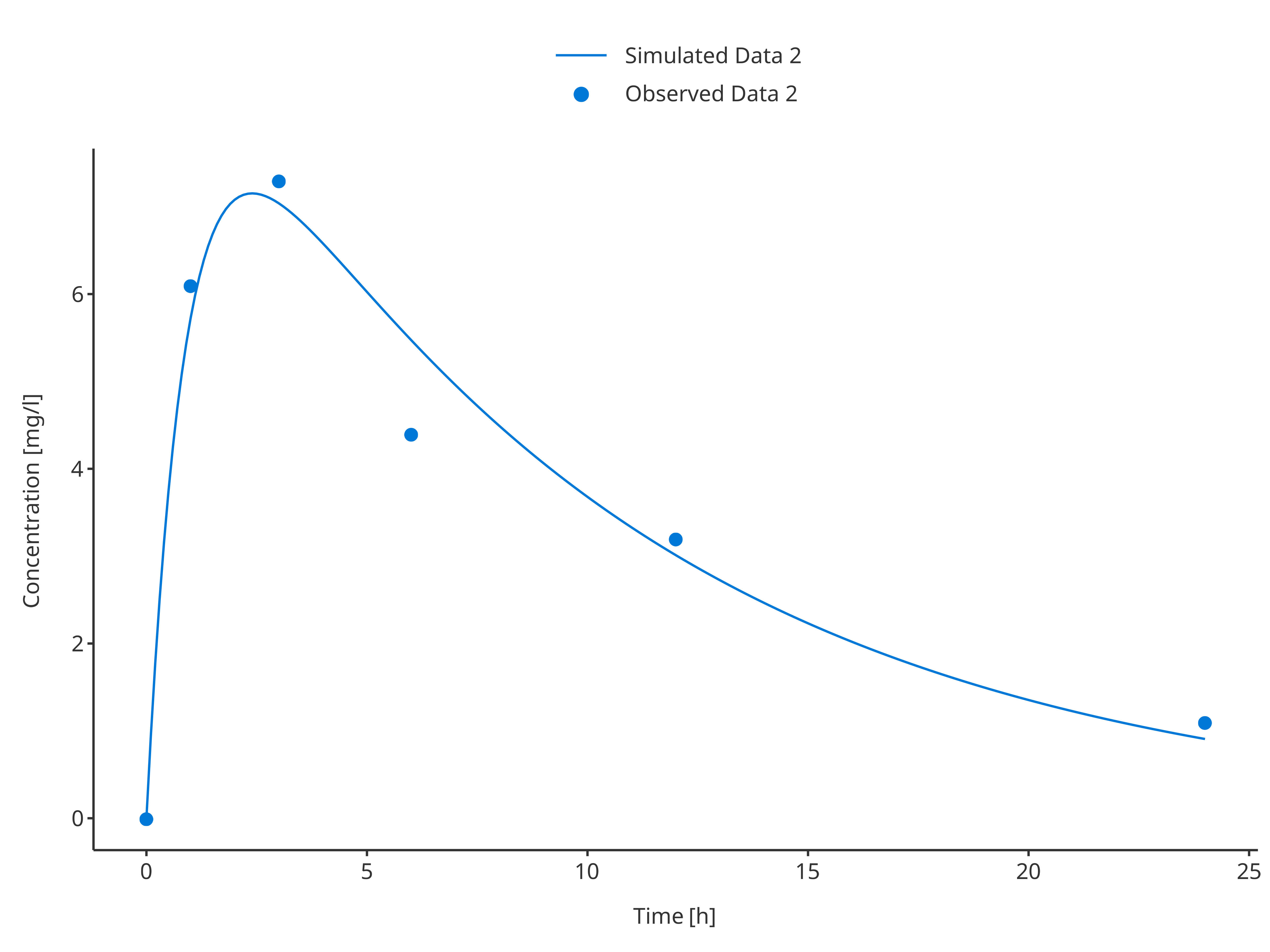
plotTimeProfile(
  data = simData2,
  observedData = obsData2,
  metaData = metaData,
  dataMapping = simDataMapping,
  observedDataMapping = obsDataMapping
)
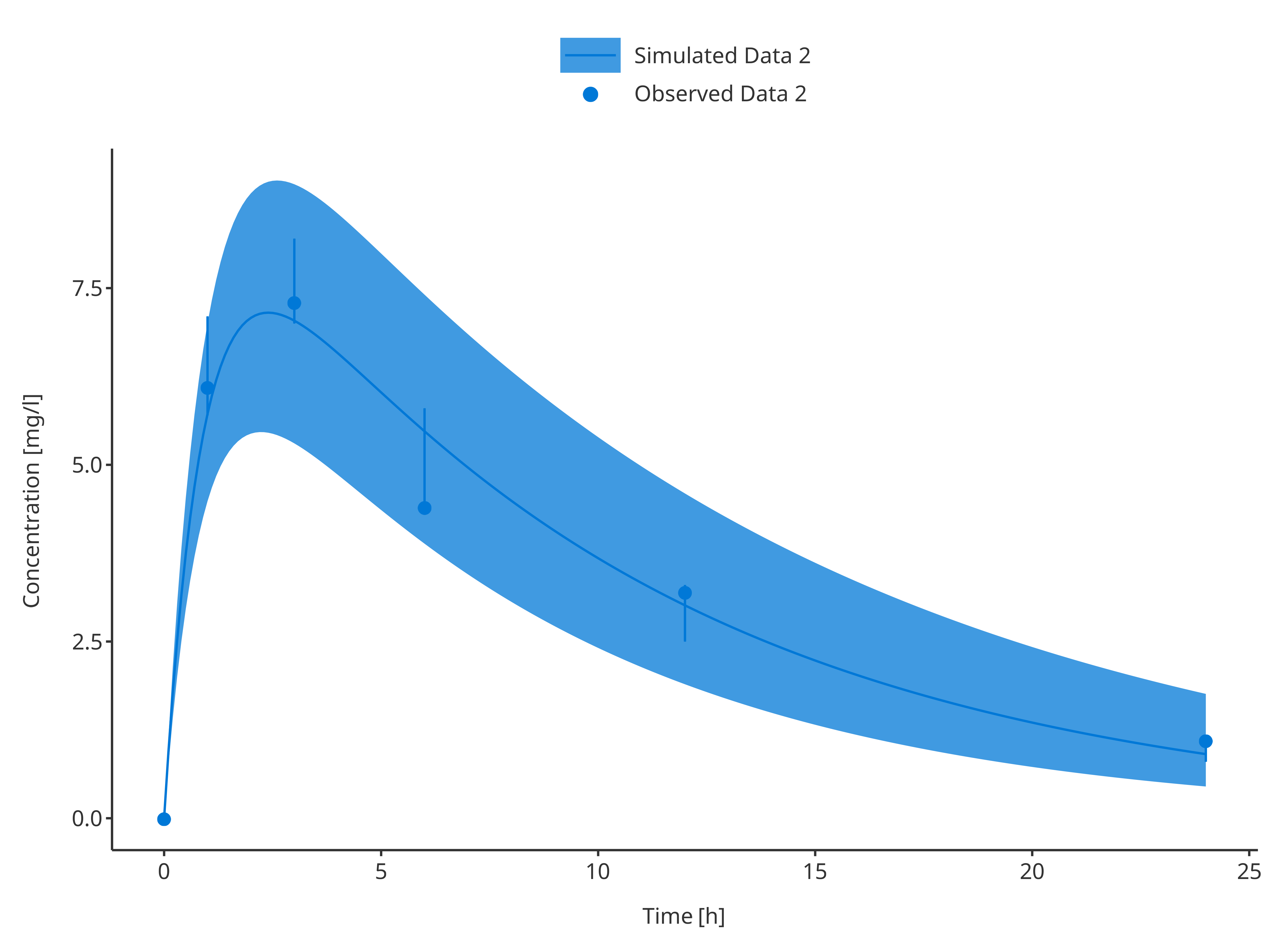
3.3.2. Single simulation and observed data set with their confidence intervals
# Define Data Mappings
simDataMapping <- TimeProfileDataMapping$new(
  x = "time",
  y = "concentration",
  ymin = "minConcentration",
  ymax = "maxConcentration",
  group = "caption"
)

obsDataMapping <- ObservedDataMapping$new(
  x = "time",
  y = "concentration",
  ymin = "minConcentration",
  ymax = "maxConcentration",
  group = "caption"
)

plotTimeProfile(
  data = simData1,
  observedData = obsData1,
  metaData = metaData,
  dataMapping = simDataMapping,
  observedDataMapping = obsDataMapping
)
plotTimeProfile(
  data = simData2,
  observedData = obsData2,
  metaData = metaData,
  dataMapping = simDataMapping,
  observedDataMapping = obsDataMapping
)
3.3.3. Multiple simulations and observed data sets
Combining multiple simulations and/or observed data sets is rather simple. To differentiate between the simulations/data sets, a grouping variable corresponding to the legend caption needs to be defined as illustrated below.
# Define Data Mappings
simDataMapping <- TimeProfileDataMapping$new(
  x = "time",
  y = "concentration",
  group = "caption"
)

obsDataMapping <- ObservedDataMapping$new(
  x = "time",
  y = "concentration",
  group = "caption"
)

simAndObsTimeProfile <- plotTimeProfile(
  data = rbind.data.frame(
    simData1,
    simData2
  ),
  observedData = rbind.data.frame(
    obsData1,
    obsData2
  ),
  metaData = metaData,
  dataMapping = simDataMapping,
  observedDataMapping = obsDataMapping
)
simAndObsTimeProfile
In this example observed and simulated data do not share any mapping. Therefore, their color pattern may not match. To update the plot and have appropriate colors and labels in the legend, it is possible to get the legend properties and update them as illustrated in the example below that updates the positions of the legend entries:
plotLegend <- getLegendCaption(simAndObsTimeProfile)
knitr::kable(as.data.frame(plotLegend$color))| names | labels | values |
|---|---|---|
| Simulated Data 1 | Simulated Data 1 | #0078D7 |
| Simulated Data 2 | Simulated Data 2 | #D83B01 |
| Observed Data 1 | Observed Data 1 | #0078D7 |
| Observed Data 2 | Observed Data 2 | #D83B01 |
plotLegend$color <- plotLegend$color[c(1, 3, 2, 4), ]
updateTimeProfileLegend(simAndObsTimeProfile, plotLegend)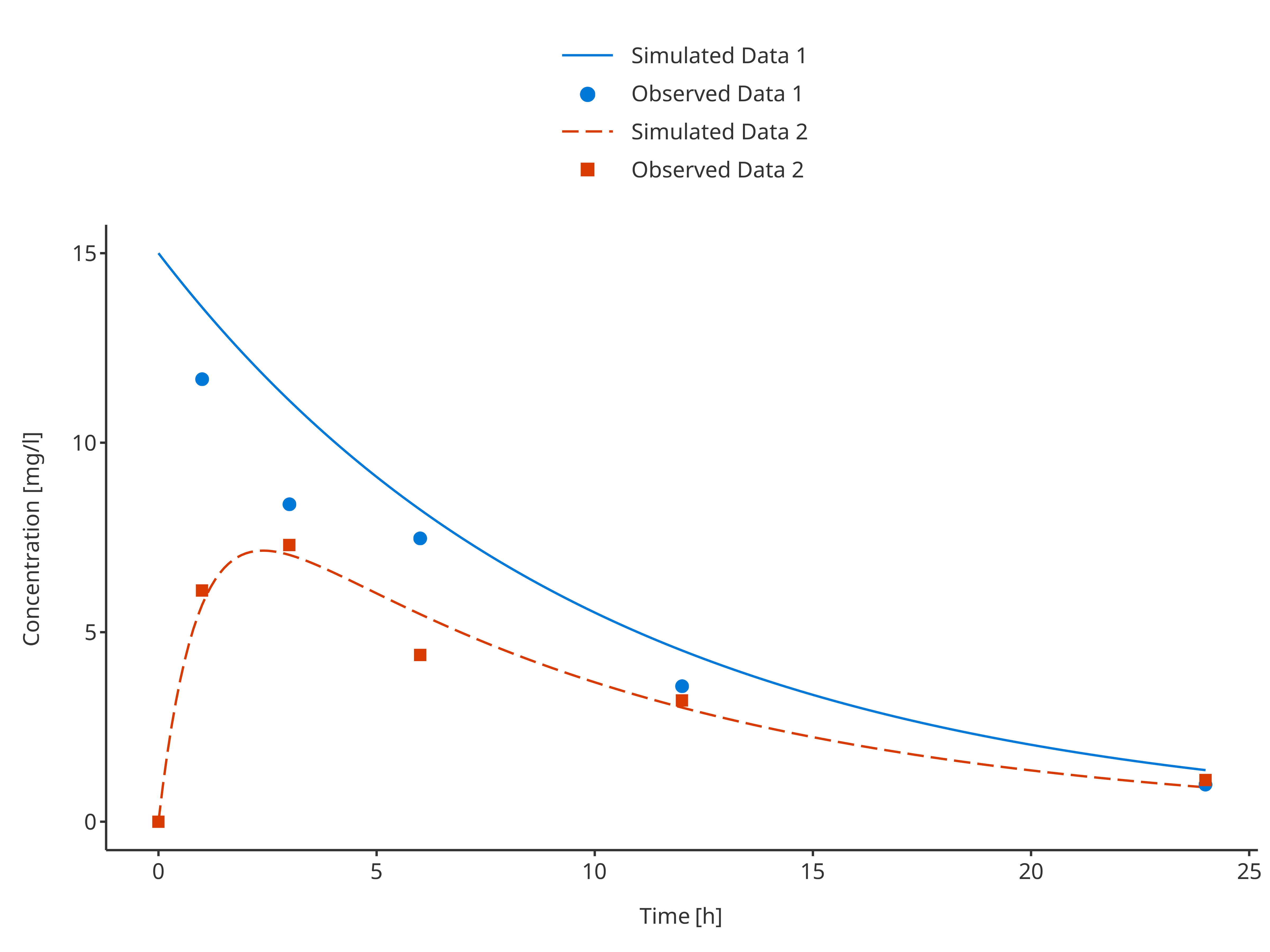
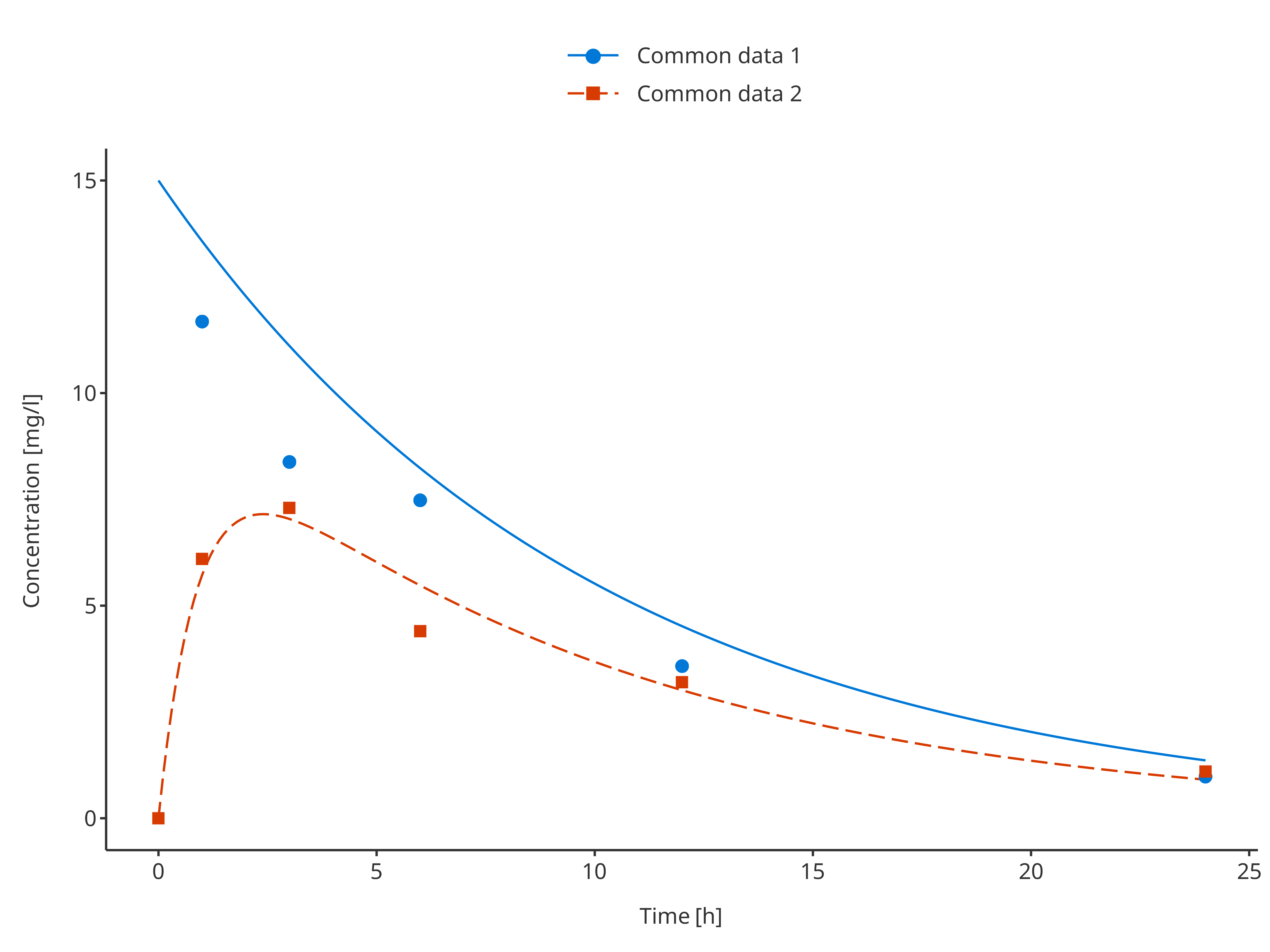
Note that if observed and simulated data share common groupings, they will be merged in the final legend.
commonSimData1 <- simData1
commonObsData1 <- obsData1
commonSimData1$caption <- "Common data 1"
commonObsData1$caption <- "Common data 1"
commonSimData2 <- simData2
commonObsData2 <- obsData2
commonSimData2$caption <- "Common data 2"
commonObsData2$caption <- "Common data 2"

plotTimeProfile(
  data = rbind.data.frame(commonSimData1, commonSimData2),
  observedData = rbind.data.frame(commonObsData1, commonObsData2),
  metaData = metaData,
  dataMapping = simDataMapping,
  observedDataMapping = obsDataMapping
)
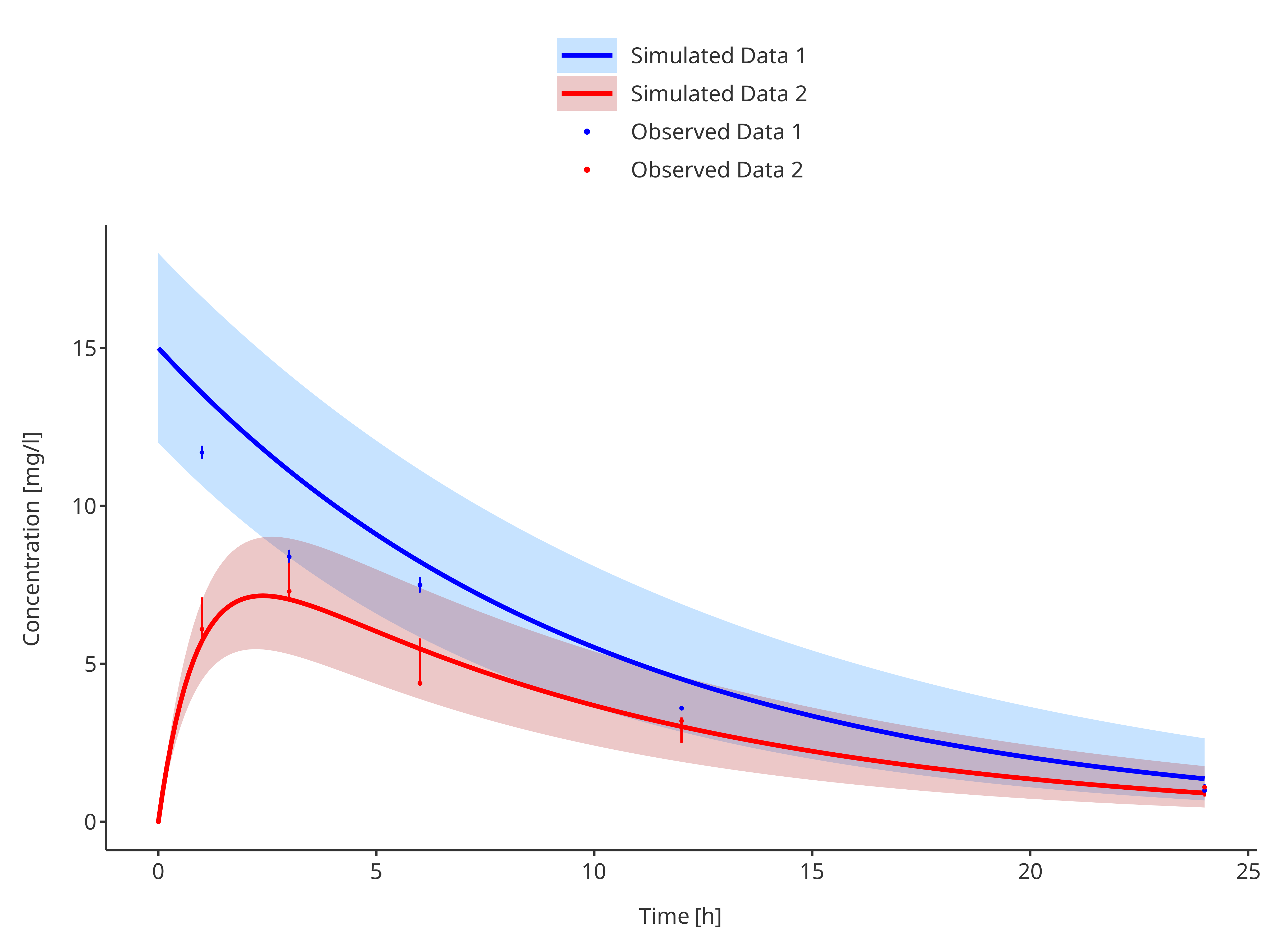
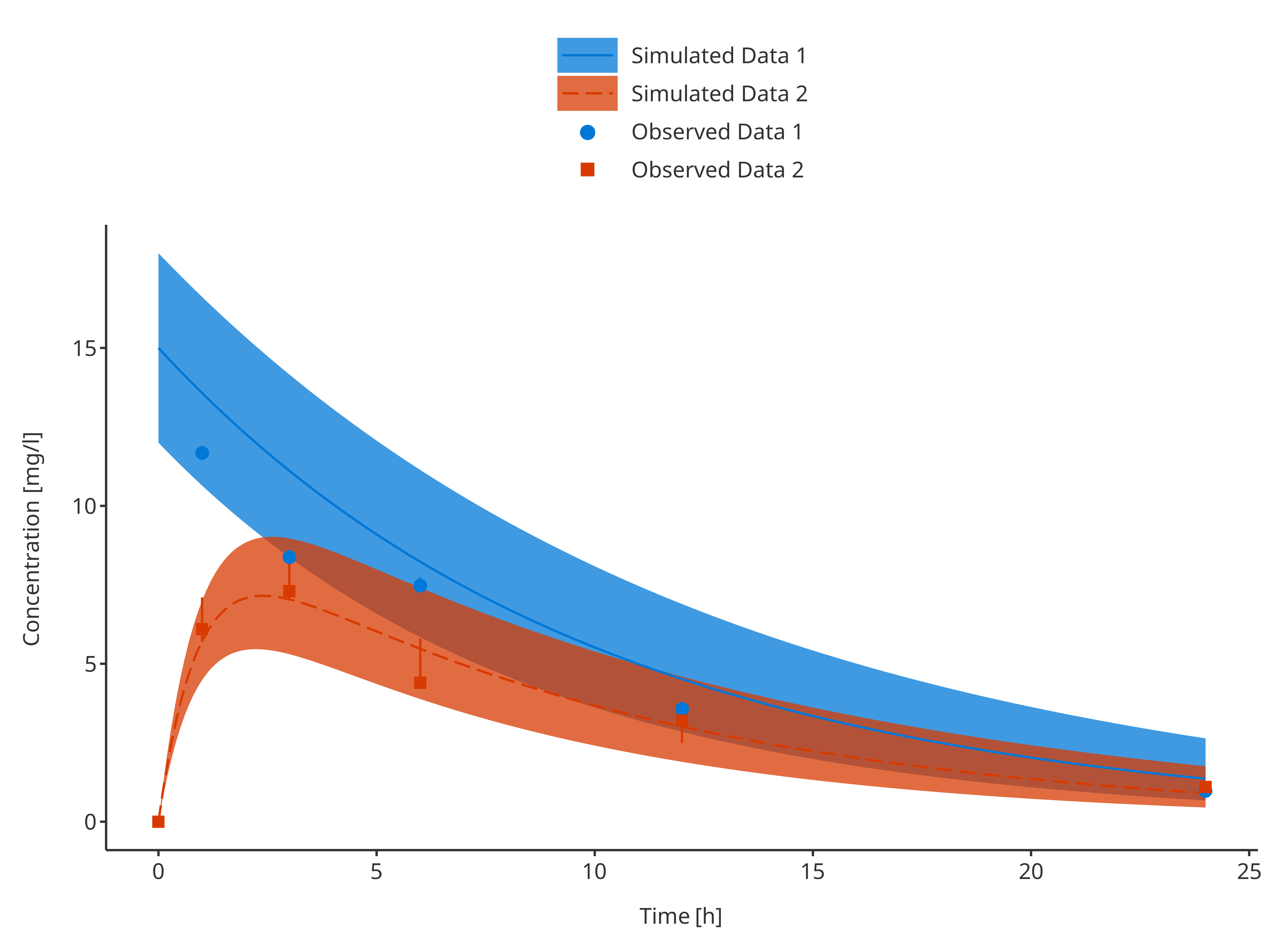
3.3.4. Multiple simulations and observed data sets with their confidence intervals
# Define Data Mappings
simDataMapping <- TimeProfileDataMapping$new(
  x = "time",
  y = "concentration",
  ymin = "minConcentration",
  ymax = "maxConcentration",
  group = "caption"
)

obsDataMapping <- ObservedDataMapping$new(
  x = "time",
  y = "concentration",
  ymin = "minConcentration",
  ymax = "maxConcentration",
  group = "caption"
)

plotTimeProfile(
  data = rbind.data.frame(
    simData1,
    simData2
  ),
  observedData = rbind.data.frame(
    obsData1,
    obsData2
  ),
  metaData = metaData,
  dataMapping = simDataMapping,
  observedDataMapping = obsDataMapping
)
3.4. Plot Configuration
For time profile plot properties can be defined in advance using
TimeProfilePlotConfiguration objects.
The code below defines a smart plot configuration that uses
data, metaData, and dataMapping
to define the names of labels.
tpConfiguration <- TimeProfilePlotConfiguration$new(
  data = simData1,
  metaData = metaData,
  dataMapping = simDataMapping
)
As every PlotConfiguration objects,
TimeProfilePlotConfiguration objects include fields
defining the properties of its lines, points,
ribbons and errorbars. By default, these
properties are used from the current theme, but can be overridden as
illustrated below.
# Define which lines are used for simulated data
tpConfiguration$lines$linetype <- Linetypes$solid
tpConfiguration$lines$size <- 1
tpConfiguration$lines$color <- c("blue", "red")

# Define which ribbons are used for simulated data CI
tpConfiguration$ribbons$fill <- c("dodgerblue", "firebrick")
tpConfiguration$ribbons$alpha <- 0.25

# Define which shapes are used for observed data
tpConfiguration$points$shape <- Shapes$circle
tpConfiguration$points$size <- 1
tpConfiguration$points$color <- c("blue", "red")

# Define which errorbars are used for observed data CI
tpConfiguration$errorbars$color <- "black"
tpConfiguration$errorbars$size <- 0.5
The corresponding plot is shown below:
plotTimeProfile(
  data = rbind.data.frame(
    simData1,
    simData2
  ),
  observedData = rbind.data.frame(
    obsData1,
    obsData2
  ),
  metaData = metaData,
  dataMapping = simDataMapping,
  observedDataMapping = obsDataMapping,
  plotConfiguration = tpConfiguration
)