1. Introduction
1.1. Objectives
The aim of this vignette is to document and illustrate the typical
workflow needed for the production of plots using the
tlf-library.
1.2. Libraries
The main purpose of the tlf-library is to standardize
the production of ggplot objects from data produced by the
OSPSuiteR package. As such, tlf-library
requires that the ggplot2 package be installed.
1.3. tlf typical workflow
The suggested workflow for producing any kind of plot with the
tlf-library is illustrated in the figure below.
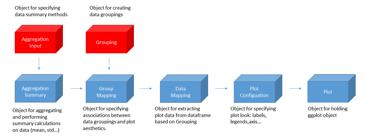
The standard workflow then proceeds as follows:
Step 0 - Data gathering. Gather the data into tidy
data.frame format.
Step 1 - Data pre-processing Pre-process the data
using AggregationSummary class.
Step 2 - Data grouping Use the
GroupMapping class to specify groupings according to which
the data will be captioned in figure legends.
Step 3 - Data mapping. Use the
DataMapping class to select the independent and dependent
variables of the processed data as well as the aesthetics that will be
used to differentiate between the groupings of the data that were
specified in step 2.
Step 4 - Plot configuration Set the
PlotConfiguration object which will define settings of the
plot such as axis labeling, font sizes, and watermarks.
Step 5 - Plot generation Create a
ggplot object from the above classes using the dedicated
plotting function.
Steps 1, 2, 3, and 4 are not mandatory. If they are skipped,
tlf-library uses default settings in lieu of the objects
created otherwise. Additionally, the PlotConfiguration
object and the DataMapping object can be created
independently. Sections 2 to 4 will focus on
AggregationSummary, DataMapping, and
PlotConfiguration.
1.4. Naming Conventions
In this package, it was chosen to use specific names for functions
and classes referring to specific plots. The naming convention for
classes is <Plot Name><Class> and for function
<function><Plot Name>. Below presents the table
of specific classes and functions that are created using this
convention:
| DataMapping | PlotConfiguration | plot | |
|---|---|---|---|
| PKRatio | PKRatioDataMapping | PKRatioPlotConfiguration | plotPKRatio |
| DDIRatio | DDIRatioDataMapping | DDIRatioPlotConfiguration | plotDDIRatio |
| IndividualIdProfile | IndividualIdProfileDataMapping | IndividualIdProfilePlotConfiguration | plotIndividualIdProfile |
| ObsVsPred | ObsVsPredDataMapping | ObsVsPredPlotConfiguration | plotObsVsPred |
| Histogram | HistogramDataMapping | HistogramPlotConfiguration | plotHistogram |
| BoxWhisker | BoxWhiskerDataMapping | BoxWhiskerPlotConfiguration | plotBoxWhisker |
2. Data pre-processing: AggregationSummary class
2.1. Data format
The workflow assumes that the data to be plotted has been gathered in the form of a tidy dataframe. In a tidy format dataframe, each measurement, such as a simulation result or an experimental observation, is described entirely in one row. The columns of the data.frame are limited to no more than the independent variable columns of the measurement (for example, time and IndividualId) and the dependent variable columns (in this case Organism|VenousBlood|Volume), which hold the value of the measurement. Since no additional columns are allowed, two dependent variables that have differing sets of independent variables should each have their own tidy dataframes.
In the sequel, we will use a dataset derived from the
OSPSuiteR package: testData. Let’s look at a
few rows to get a sense of the data:
| IndividualId | Gender | Race | Population Name | Organism|Age | Organism|Weight |
|---|---|---|---|---|---|
| 0 | Male | Caucasian | pop_10 | 14.06889 | 54.04230 |
| 1 | Male | Caucasian | pop_10 | 23.41955 | 61.29773 |
| 2 | Male | Caucasian | pop_10 | 24.89981 | 44.39078 |
| 3 | Male | Caucasian | pop_10 | 30.45043 | 53.61099 |
| 4 | Male | Caucasian | pop_10 | 22.96949 | 42.98250 |
| 5 | Female | Caucasian | pop_10 | 37.71187 | 50.49205 |
2.2. MetaData
A metaData variable associated with the data can be used
to define additional information such as the dimension and
unit of each column in the data.frame. The
lower limit of quantification of a IndividualId profile can also be
stored in the metaData. The format of metaData is currently
expected to be a list on each variable of lists showing unit and
dimension.
| Variable | Dimension | Unit |
|---|---|---|
| IndividualId | ||
| Gender | ||
| Race | ||
| Population Name | ||
| Organism|Age | Age | yrs |
| Organism|Weight | Mass | kg |
| Organism|BMI | kg/m2 | |
| Organism|Gestational age | Age | week(s) |
| Organism|Height | Length | dm |
| Organism|Hematocrit | Volume | l |
| Organism|VenousBlood|Volume | Volume | l |
| Organism|ArterialBlood|Volume | Volume | l |
| Organism|Bone|Specific blood flow rate | Flow | l/min |
| Organism|Bone|Volume | Volume | l |
| Organism|Brain|Volume | Volume | l |
| Compound | ||
| Dose | Mass | mg |
2.3. Aggregation
A common processing of the data is its aggregation. The aggregation consists in splitting the data into subsets, then computing summary statistics for each, and returning the result in a convenient form. Visual predictive checks are typical plots where such method is useful.
The AggregationSummary class is a helper class that
simplifies the use of aggregation methods on the data. The
R6 class AggregationSummary automates the
computation of multiple summary statistics of the raw data produced at
Step 0. The output of this optional data pre-processing
step is a dataframe with a column for each summary statistic. This
dataframe can be input into the subsequent steps of the workflow. The
user also has the option of generating metaData for each of
the summary statistics evaluated.
To illustrate the functions of this class for the example of the
dataframe testData, let’s suppose that for each individual
in the IndividualId column, the minimum and the
mean value of the simulated
Organism|VenousBlood|Volume column is to be computed for each
gender in the Gender column. The
AggregationSummary class works in 3 steps:
Three sets of columns are selected from the input dataframe
data: an independent variable set calledxColumnNames(in this case, the IndividualId column intestData), a grouping variables set calledgroupingColumnNames(the Gender column intestData) and a dependent variables set calledyColumnNames(the Organism|VenousBlood|Volume column intestData).For each value of the independent variable
xColumnNames, the rows of the dataframe are aggregated into groups defined by unique combinations of the elements in the grouping variable columnsgroupingColumnNames.Summary statistics (in this case, the
minimumand themean) for theyColumnNamesvariables in each group are evaluated. The functions for computing the the summary statistics are specified when initializing anAggregationSummary, viaaggregationFunctionsVector. User-specified descriptive names of these functions are supplied via the vector of strings namedaggregationFunctionNames. The units and dimensions of the outputs of these functions are supplied via the vectors of strings namedaggregationUnitsVectorandaggregationDimensionsVector, respectively.
For this example, the AggregationSummary object
aggSummary is instantiated as follows:
aggSummary <- AggregationSummary$new(
  data = testData,
  metaData = testMetaData,
  xColumnNames = "IndividualId",
  groupingColumnNames = "Gender",
  yColumnNames = "Organism|VenousBlood|Volume",
  aggregationFunctionsVector = c(min, mean),
  aggregationFunctionNames = c(
    "Simulated Min",
    "Simulated Mean"
  ),
  aggregationUnitsVector = c("l", "l"),
  aggregationDimensionsVector = c(
    "Volume",
    "Volume"
  )
)
The dataframe that holds the summary statistics of the aggregated
rows is stored in the dfHelper property of the resulting
aggSummary object. Since two functions (min
and mean) were specified in
aggregationFunctionsVector, the dataframe
aggSummary$dfHelper has, in addition to the
xColumnNamesand groupingColumnNames columns,
two additional columns named Simulated Min and
Simulated Mean, which were the names specified in
aggregationFunctionNames.
head(aggSummary$dfHelper)| IndividualId | Gender | Simulated Min | Simulated Mean |
|---|---|---|---|
| 5 | Female | 0.6186527 | 0.6186527 |
| 6 | Female | 0.6700546 | 0.6700546 |
| 7 | Female | 0.8003464 | 0.8003464 |
| 8 | Female | 0.6001890 | 0.6001890 |
| 9 | Female | 0.7350718 | 0.7350718 |
| 0 | Male | 0.8767134 | 0.8767134 |
The metaData corresponding to the columns of the
resulting dataframes are lists that are stored together in a list with
the metaData of the xColumnNamesand
groupingColumnNames columns. The metaData for
the new aggSummary$dfHelper dataframe is stored as the
metaDataHelper property of the aggSummary
object. For this example, the two metaData lists
corresponding to the Simulated Min and
Simulated Mean columns are also are labeled
Simulated Min and Simulated Mean. The contents
of the list aggSummary$metaDataHelper are:
# Currently issue with metaData of Gender
aggSummary$metaDataHelper[[2]] <- NULL
aggMetaData <- data.frame(
  "unit" = sapply(aggSummary$metaDataHelper, function(x) {
    x$unit
  }),
  "dimension" = sapply(aggSummary$metaDataHelper, function(x) {
    x$dimension
  })
)

knitr::kable(aggMetaData)| unit | dimension | |
|---|---|---|
| IndividualId | ||
| Simulated Min | l | Volume |
| Simulated Mean | l | Volume |
3. Mapping and grouping of data: DataMapping class
The role of the DataMapping class is to provide a
user-friendly interface to indicate what data should be plotted. In most
cases, this class needs to be initialized to map what variables are
x and y, and which IndividualIds variable(s)
will group the data. Thus, the most common input are x and
y; however, for more advanced plots, input such as
groupMapping may be used often. For advanced plots,
subclasses are derived from DataMapping, they use unique
input and default related to the advanced plot to make it easier to use
them.
3.1. GroupMapping
3.1.1. Grouping class
An R6 class called Grouping can be used to
group the data into subsets that, in the final plots, are to be
distinguished both aesthetically and in legend captions. In addition,
these subsets can be listed under descriptive legend titles.
As an example, a Grouping object called
grouping1 can be used to specify that the data in a
tidy data.frame should be grouped by both “Compound” and
“Dose”:
With this minimal input, a legend associated with this grouping will
have the default title “Compound-Dose”. On the other hand, a custom
title for this grouping and its legend can be supplied by the user with
the optional label input:
# Grouping by variable names and overwriting the default label:
grouping2 <- Grouping$new(group = c("Compound", "Dose"), label = "Compound & Dose")
In the above two examples, default captions are constructed by
hyphenating the compound type and the dose amount for each row.
Alternatively, the captions can be customized by the user by supplying a
dataframe with the custom captions to the group input of
the Grouping object constructor. The format of this
dataframe is such that the rightmost column contains the desired
captions, the name of this rightmost column is the default legend title
for this grouping, and the remaining columns define the combinations of
row entries that are to receive each caption in the rightmost column. To
illustrate this method, the following dataframe
mappingDataFrame is used to assign captions based on
entries in the “Dose” and “Compound” columns. For example, the caption
“6mg of Aspirin” is assigned to any row in which the “Dose” entry is 6
and the “Compound” entry is “Aspirin”.
# Grouping using a data.frame:
mappingDataFrame <- data.frame(
  Compound = c("Aspirin", "Aspirin", "Sugar", "Sugar"),
  Dose = c(6, 3, 6, 3),
  "Compound & Dose" = c(
    "6mg of Aspirin",
    "3mg of Aspirin",
    "6mg of Sugar",
    "3mg of Sugar"
  ),
  check.names = FALSE
)
knitr::kable(mappingDataFrame)| Compound | Dose | Compound & Dose |
|---|---|---|
| Aspirin | 6 | 6mg of Aspirin |
| Aspirin | 3 | 3mg of Aspirin |
| Sugar | 6 | 6mg of Sugar |
| Sugar | 3 | 3mg of Sugar |
grouping3 <- Grouping$new(group = mappingDataFrame)The default title of the legend that results from this grouping is
the name of the rightmost column, which is “Compound & Dose”. Note
that the check.names option should be set to
FALSE when creating the dataframe
mappingDataFrame, since the legend title contains spaces in
this instance. This legend title can be overridden to be another string
by using the label input of the object constructor, as in
the case of grouping2 above.
The three Grouping objects, grouping1,
grouping2, and grouping3 respectively yield
the last three columns of the following dataframe:
# Apply the mapping to get the grouping captions:
groupingsDataFrame <- data.frame(
  testData$IndividualId,
  testData$Dose,
  testData$Compound,
  grouping1$getCaptions(testData),
  grouping2$getCaptions(testData),
  grouping3$getCaptions(testData)
)

names(groupingsDataFrame) <- c(
  "IndividualId", "Dose", "Compound",
  grouping1$label, grouping2$label, grouping3$label
)

# Show results for all groupings:
knitr::kable(groupingsDataFrame)| IndividualId | Dose | Compound | Compound-Dose | Compound & Dose | Compound & Dose |
|---|---|---|---|---|---|
| 0 | 6 | Aspirin | Aspirin-6 | Aspirin-6 | 6mg of Aspirin |
| 1 | 3 | Aspirin | Aspirin-3 | Aspirin-3 | 3mg of Aspirin |
| 2 | 6 | Aspirin | Aspirin-6 | Aspirin-6 | 6mg of Aspirin |
| 3 | 3 | Sugar | Sugar-3 | Sugar-3 | 3mg of Sugar |
| 4 | 6 | Sugar | Sugar-6 | Sugar-6 | 6mg of Sugar |
| 5 | 3 | Aspirin | Aspirin-3 | Aspirin-3 | 3mg of Aspirin |
| 6 | 6 | Aspirin | Aspirin-6 | Aspirin-6 | 6mg of Aspirin |
| 7 | 3 | Sugar | Sugar-3 | Sugar-3 | 3mg of Sugar |
| 8 | 6 | Sugar | Sugar-6 | Sugar-6 | 6mg of Sugar |
| 9 | 3 | Sugar | Sugar-3 | Sugar-3 | 3mg of Sugar |
A dataframe can also be used to create a Grouping object
that subsets the data based on whether a numeric grouping variable
satisfies an specific inequality. For example, individuals in
testData can be grouped according to whether or not their
age exceeds 6 years by first defining the following dataframe:
# Grouping using a data.frame:
binningDataFrame <- data.frame(
  Age = I(list(c(0, 6), c(7, 100))),
  "Age Range" = c(
    "Age 6 or lower",
    "Above age 6"
  ),
  check.names = FALSE
)
Then creating a new grouping:
grouping4 <- Grouping$new(group = binningDataFrame)This new Grouping object grouping4 yields
the following captions
# Apply the mapping to get the grouping captions:
testData$Age <- testData$`Organism|Age`
binnedGroupingsDataFrame <- data.frame(
  testData$IndividualId,
  testData$Age,
  grouping4$getCaptions(testData)
)

names(binnedGroupingsDataFrame) <- c("IndividualId", "Age", grouping4$label)

# Show results for all groupings:
knitr::kable(binnedGroupingsDataFrame)| IndividualId | Age | Age Range |
|---|---|---|
| 0 | 14.06889 | Above age 6 |
| 1 | 23.41955 | Above age 6 |
| 2 | 24.89981 | Above age 6 |
| 3 | 30.45043 | Above age 6 |
| 4 | 22.96949 | Above age 6 |
| 5 | 37.71187 | Above age 6 |
| 6 | 50.12875 | Above age 6 |
| 7 | 32.53951 | Above age 6 |
| 8 | 26.86401 | Above age 6 |
| 9 | 45.97137 | Above age 6 |
3.1.2. GroupMapping class
An additional R6 class called GroupMapping
maps Grouping objects to aesthetic parameters such as
color or linetype. To distinguish between
“Compound” and “Dose” groups by color and to use the captions and legend
title specified in grouping2, the following groupings
object groups1 is constructed:
# Map groups to aesthetic properties
groups1 <- GroupMapping$new(color = grouping2)
A GroupMapping object groups2 can also be
constructed more quickly by directly associating an aesthetic, such as
color, to a vector of dataframe column names:
# Map groups to aesthetic properties
groups2 <- GroupMapping$new(color = c("Compound", "Dose"))
or to a Grouping object directly:
# Map groups to aesthetic properties
groups3 <- GroupMapping$new(color = Grouping$new(
  group = c("Compound", "Dose"),
  label = c("Compound & Dose")
))
3.2. DataMapping
The R6 class XYGDataMapping extracts the
maps the x, y, and grouping variables of data according to the
aesthetics specified in an input GroupMapping object. This
mapping is carried out by an internal function of this class named
checkMapData which checks if the variables indicated the
GroupMapping are included in the data. This method then
returns a simplified dataframe with the variables defined by the
dataMapping.
When no GroupMapping object is supplied upon
construction of a XYGDataMapping object, the function
checkMapData returns a dataframe with x and
y. A dummy variable named aesDefault is added
to the data.frame, its sole purpose is to allow modifications of
aesthetic properties after the creation of the ggplot object (not
possible otherwise).
tpMapping <- XYGDataMapping$new(x = "IndividualId", y = "Organism|VenousBlood|Volume")
knitr::kable(tpMapping$checkMapData(
  data = testData,
  metaData = IndividualIdProfileMetaData
))| IndividualId | Organism|VenousBlood|Volume | legendLabels |
|---|---|---|
| 0 | 0.8767134 | |
| 1 | 0.8130964 | |
| 2 | 0.8054172 | |
| 3 | 0.8048924 | |
| 4 | 0.6127810 | |
| 5 | 0.6186527 | |
| 6 | 0.6700546 | |
| 7 | 0.8003464 | |
| 8 | 0.6001890 | |
| 9 | 0.7350718 |
When a GroupMapping object is supplied upon construction
of the XYGDataMapping object, each
x,y pair is associated with a group that can
be used to distinguish the pair aesthetically in the final plot:
# Re-use the variable groups previously defined
tpMapping <- XYGDataMapping$new(
  x = "IndividualId", y = "Organism|VenousBlood|Volume",
  groupMapping = groups1
)

knitr::kable(tpMapping$checkMapData(data = testData))| IndividualId | Organism|VenousBlood|Volume | Compound & Dose | legendLabels |
|---|---|---|---|
| 0 | 0.8767134 | Aspirin-6 | Aspirin-6 |
| 1 | 0.8130964 | Aspirin-3 | Aspirin-3 |
| 2 | 0.8054172 | Aspirin-6 | Aspirin-6 |
| 3 | 0.8048924 | Sugar-3 | Sugar-3 |
| 4 | 0.6127810 | Sugar-6 | Sugar-6 |
| 5 | 0.6186527 | Aspirin-3 | Aspirin-3 |
| 6 | 0.6700546 | Aspirin-6 | Aspirin-6 |
| 7 | 0.8003464 | Sugar-3 | Sugar-3 |
| 8 | 0.6001890 | Sugar-6 | Sugar-6 |
| 9 | 0.7350718 | Sugar-3 | Sugar-3 |
A feature of XYGDataMapping class is that, in addition
to specifying a y column, the user may also supply
ymin and ymax columns that can represent the
boundaries of error bars. If only ymin and
ymax are input when constructing the
XYGDataMapping object, with y left undefined
or NULL, the default profile that will ultimately be
plotted is a range plot. If y, ymin and
ymax are all input, the default plot will be a IndividualId
profile plot with an error bar.