Histogram Plots

require(tlf)
#> Loading required package: tlf

1. Introduction

The following vignette aims at documenting and illustrating workflows for producing histograms using the function plotHistogram from the tlf package.

2. Illustration of basic histograms

2.1. Data

The data showed in the sequel is available at the following path: system.file("extdata", "test-data.csv", package = "tlf"). In the code below, the data is loaded and assigned to histData.

# Load example
histData <- read.csv(
  system.file("extdata", "test-data.csv", package = "tlf"),
  stringsAsFactors = FALSE
)

# histData
knitr::kable(utils::head(histData), digits = 2)

ID	Age	Obs	Pred	Ratio	AgeBin	Sex	Country	SD
1	48	4.00	2.90	0.72	Adults	Male	Canada	0.69
2	36	4.40	5.75	1.31	Adults	Male	Canada	0.19
3	52	2.80	2.70	0.96	Adults	Male	Canada	0.98
4	47	3.75	3.05	0.81	Adults	Male	Canada	0.59
5	0	1.95	5.25	2.69	Peds	Male	Canada	0.44
6	48	2.45	5.30	2.16	Adults	Male	Canada	0.07

2.2. `plotHistogram`

Besides, the usual tlf input arguments commonly used by the plot functions (data, metaData, dataMapping, plotConfiguration and plotObject), the function plotHistogram also includes the following optional input arguments:

x: Numeric values used in the histogram instead of data and dataMapping.
bins: Number of bins
binwidth: Width of each bin, overwriting the number of bins.
stack: Logical defining if histogram bars are stacked
distribution: Name of a distribution to fit to the data. Currently, only normal and log-normal distributions are available.

2.3. Minimal examples

Most of the time, the optional input x is convenient to assess the distribution of the data.

# Use directly x for quick histogram
plotHistogram(x = histData$Ratio)


# Use directly x and bins for quick histogram with a defined number of bins
plotHistogram(x = histData$Ratio, bins = 7)

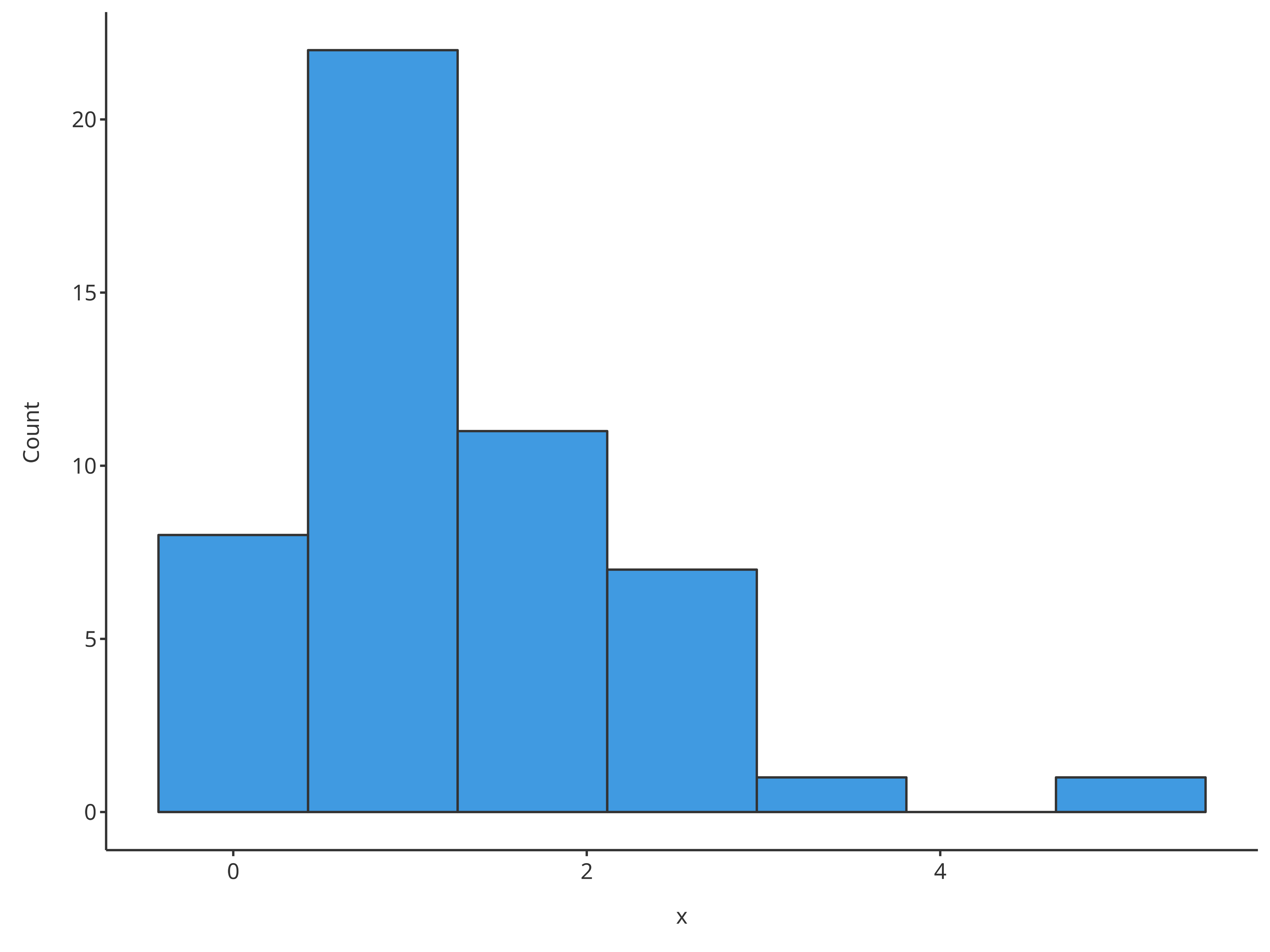
2.4. Examples using `data` and `dataMapping`

Workflows in tlf usually includes the definition of data, their metData and dataMapping.

# Create HistogramDataMapping object
histoMapping <- HistogramDataMapping$new(
  x = "Ratio",
  fill = "Sex"
)

plotHistogram(
  data = histData,
  dataMapping = histoMapping
)

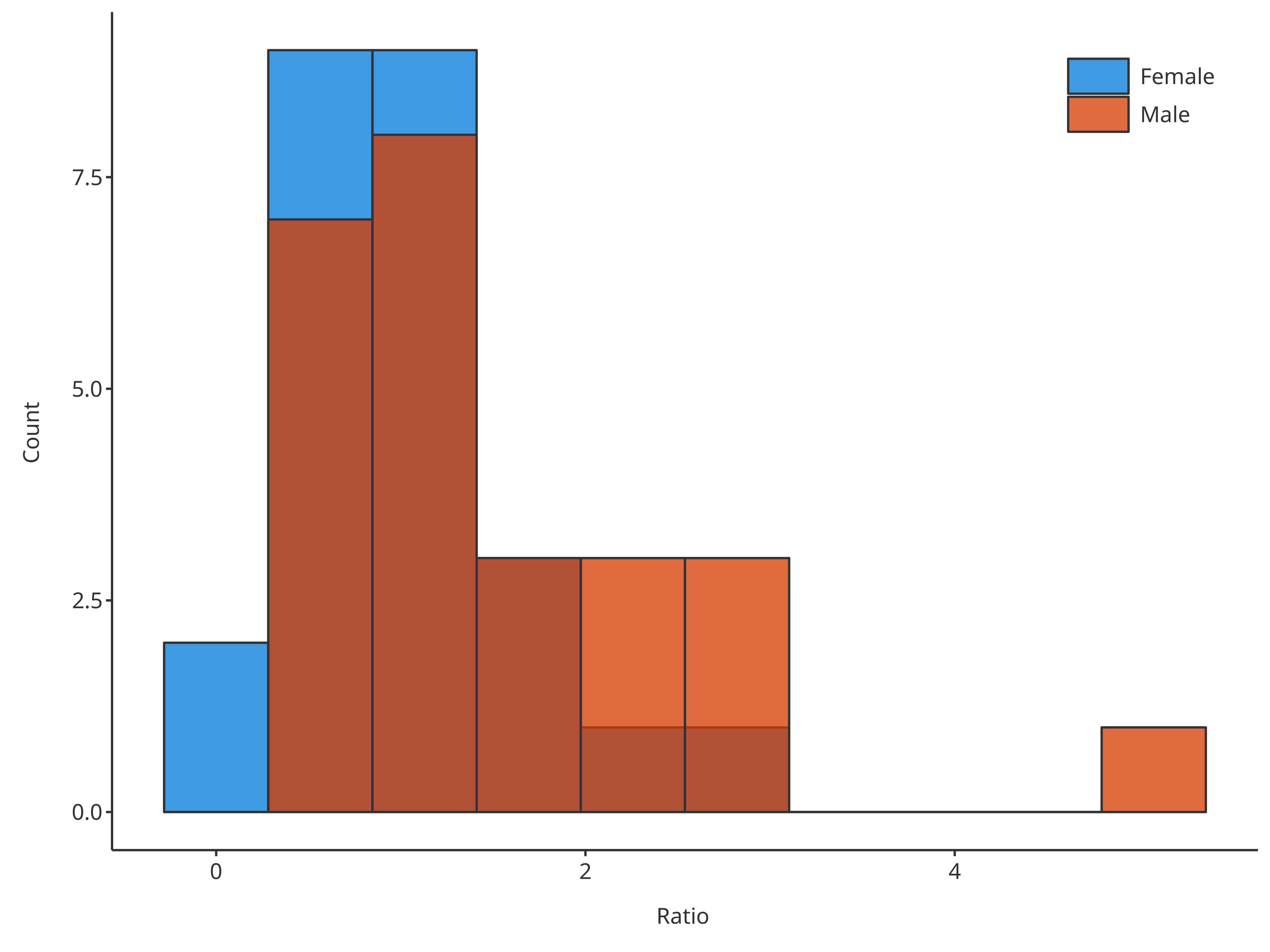
In such cases, the optional arguments previously presented can be included in dataMapping.

# Create HistogramDataMapping object
histoMapping <- HistogramDataMapping$new(
  x = "Ratio",
  fill = "Sex",
  stack = TRUE
)

plotHistogram(
  data = histData,
  dataMapping = histoMapping
)

If defined as plotHistogram input arguments, they will overwrite dataMapping.

# Create HistogramDataMapping object
histoMapping <- HistogramDataMapping$new(
  x = "Ratio",
  fill = "Sex",
  bins = 3
)

# bin defined in both, plotHistogram has priority and overwrites dataMapping internally
plotHistogram(
  data = histData,
  dataMapping = histoMapping,
  bins = 6
)

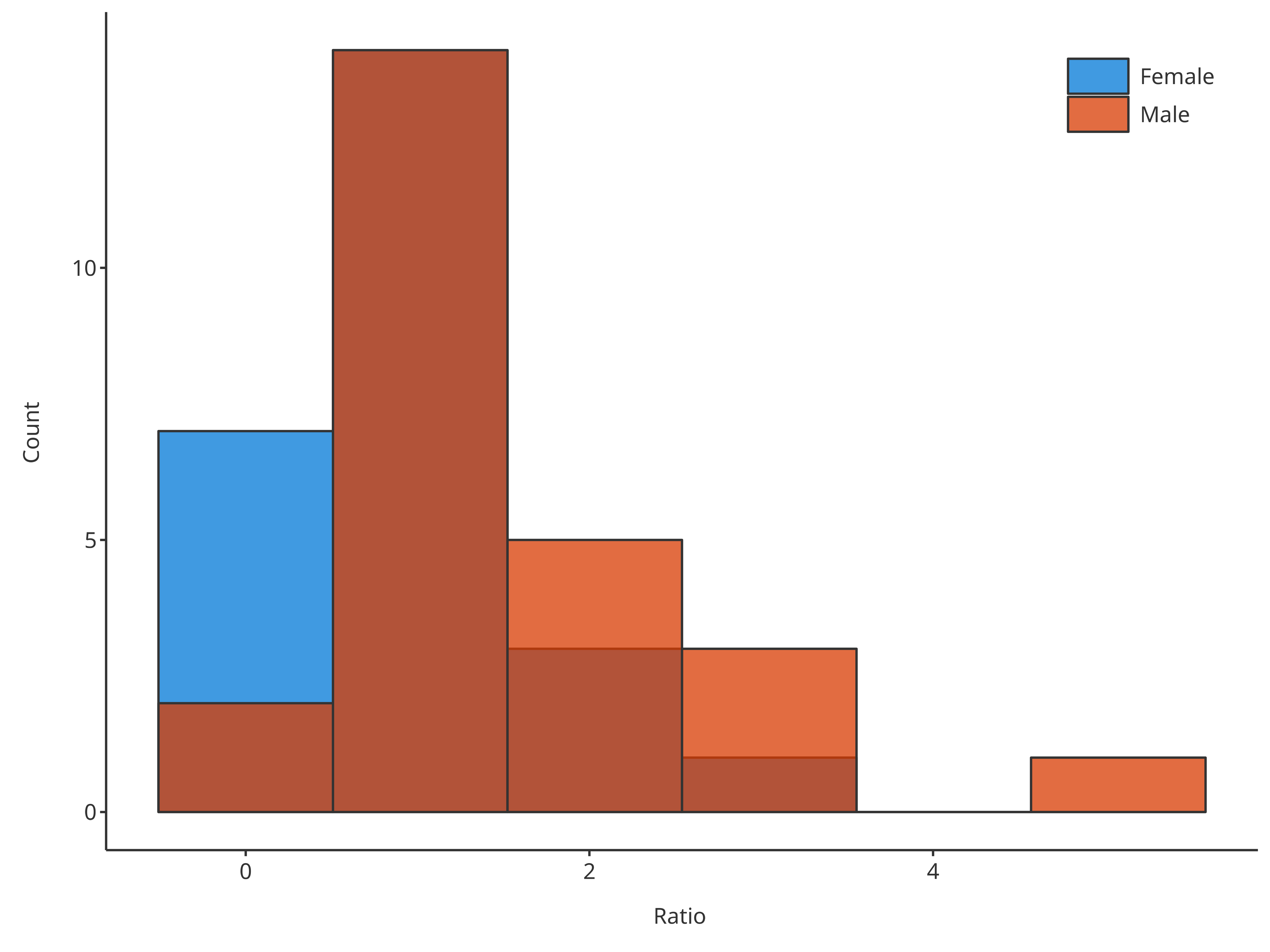
2.5. Focus on binning

There are 3 ways of defining how the data is binned. The priority between each method was defined according to their specificity. Method 1, the simplest and used as default, defines the number of bins. It can be overwritten by method 3, which defines the width of each bin. Method 2 is the more specific and defines the bin edges, consequently it cannot be overwritten by method 3.

*1. Define the number of bins with the input argument bins (using a single value)

# Create HistogramDataMapping object
histoMapping <- HistogramDataMapping$new(
  x = "Ratio",
  fill = "Sex"
)

# Define the number of bins in final plot
plotHistogram(
  data = histData,
  dataMapping = histoMapping,
  bins = 6
)

*2. Define the edges of the bins with the input argument bins (using an array of values)

# Create HistogramDataMapping object
histoMapping <- HistogramDataMapping$new(
  x = "Ratio",
  fill = "Sex"
)

# Define the edges of bins in final plot
plotHistogram(
  data = histData,
  dataMapping = histoMapping,
  bins = seq(0, 6, 0.2)
)

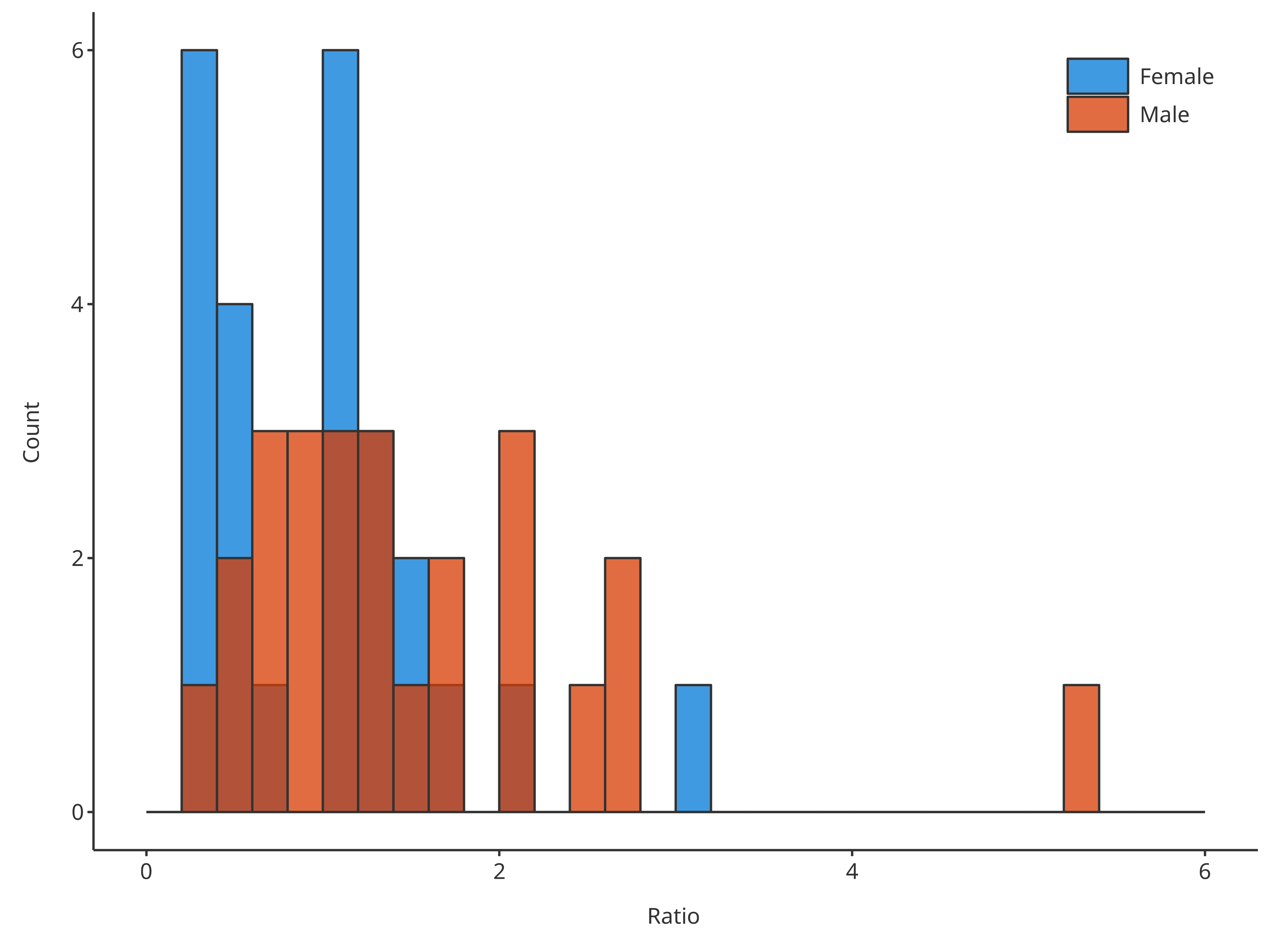
*3. Define the width of bins with the input argument binwidth (using a single value).

# Create HistogramDataMapping object
histoMapping <- HistogramDataMapping$new(
  x = "Ratio",
  fill = "Sex"
)

# Define the width of bins in final plot
plotHistogram(
  data = histData,
  dataMapping = histoMapping,
  binwidth = 0.4
)

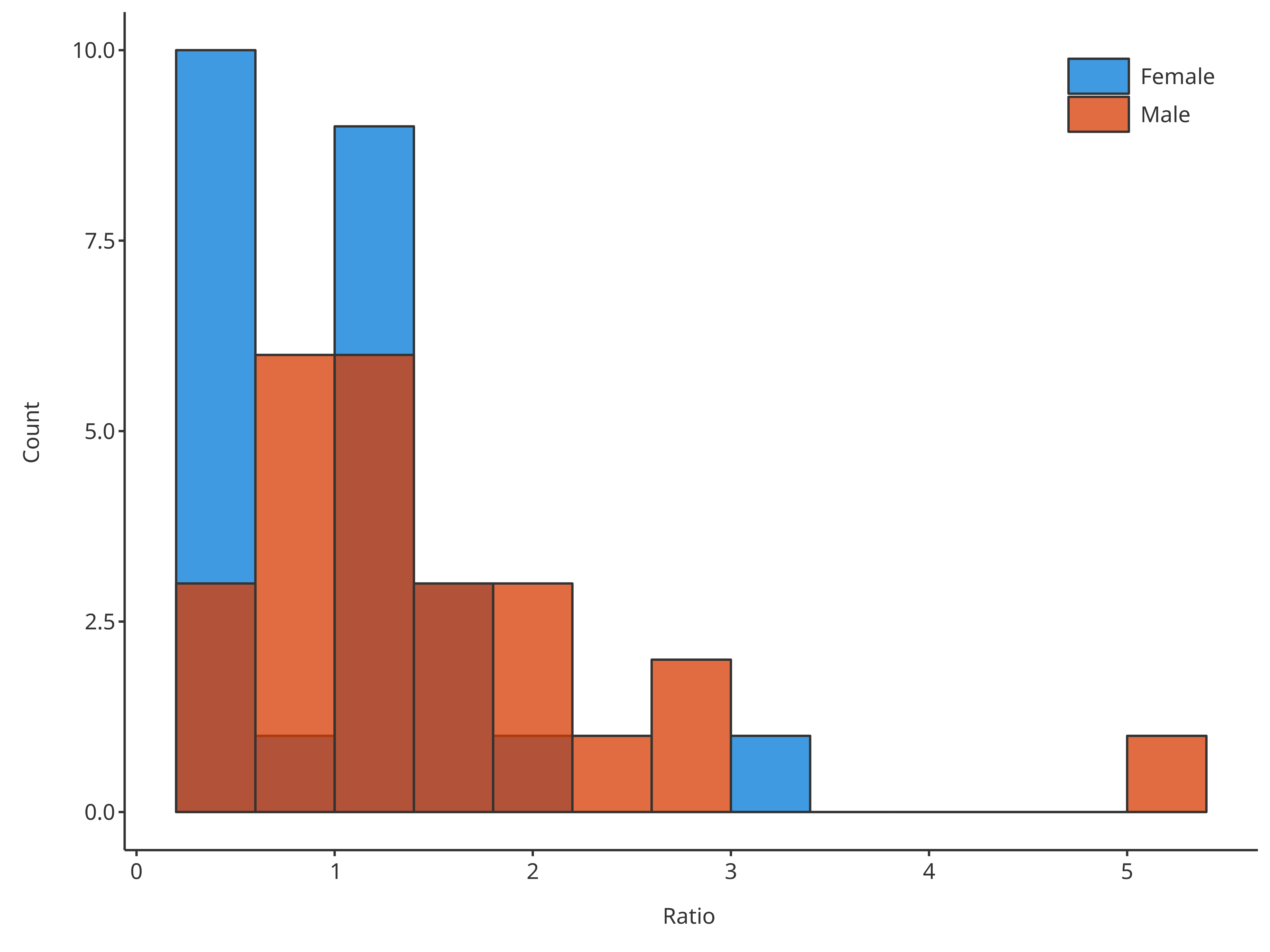
2.6. Focus on distribution fit

The optional input distribution aims at providing the possibility of fitting the data distribution. Currently, two distributions can be fitted by the function plotHistogram:

Fit a normal distribution and draw the distribution mean as vertical line using "normal"
Fit a log-normal distribution and draw the distribution mode as vertical line using "logNormal"

# Plot normal distribution
plotHistogram(
  x = histData$Ratio,
  distribution = "normal"
)


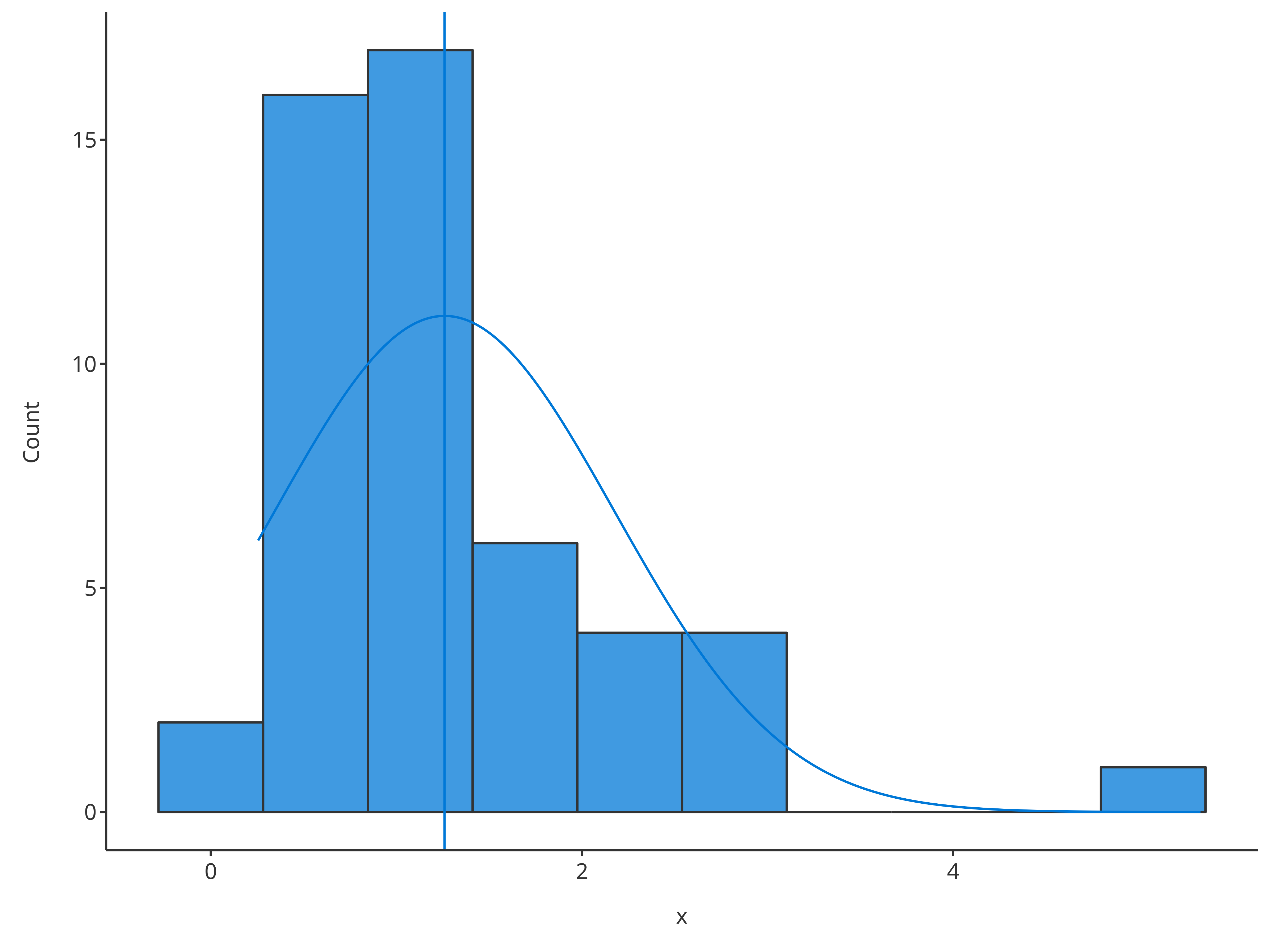
# Plot normal distribution
plotHistogram(
  x = histData$Ratio,
  distribution = "logNormal"
)

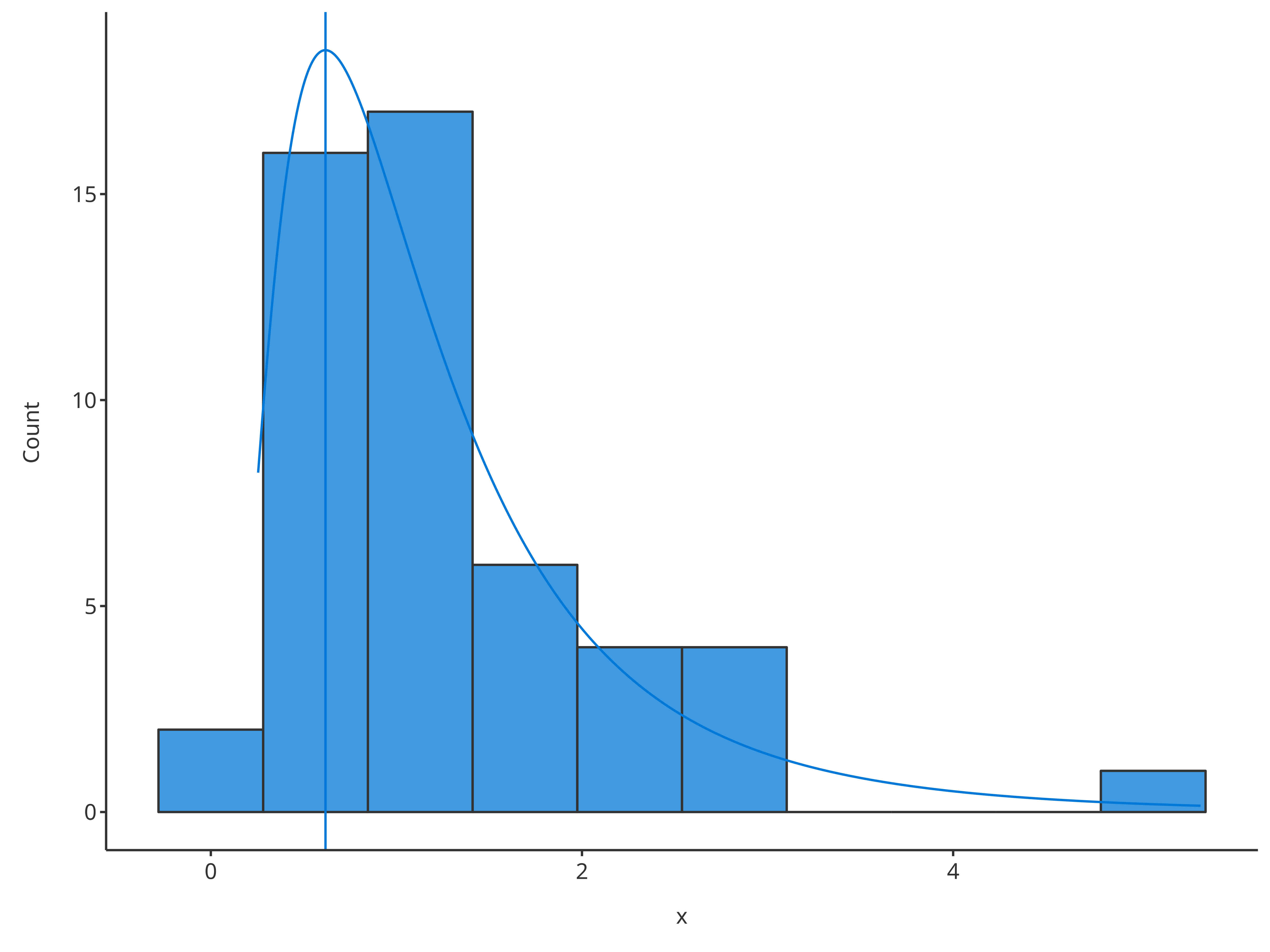
To compare multiple distributions, they can be defined through the dataMapping:

# Create HistogramDataMapping object split by gender
histoMapping <- HistogramDataMapping$new(
  x = "Ratio",
  fill = "Sex"
)

# Plot normal distribution for each gender
plotHistogram(
  data = histData,
  dataMapping = histoMapping,
  distribution = "normal"
)

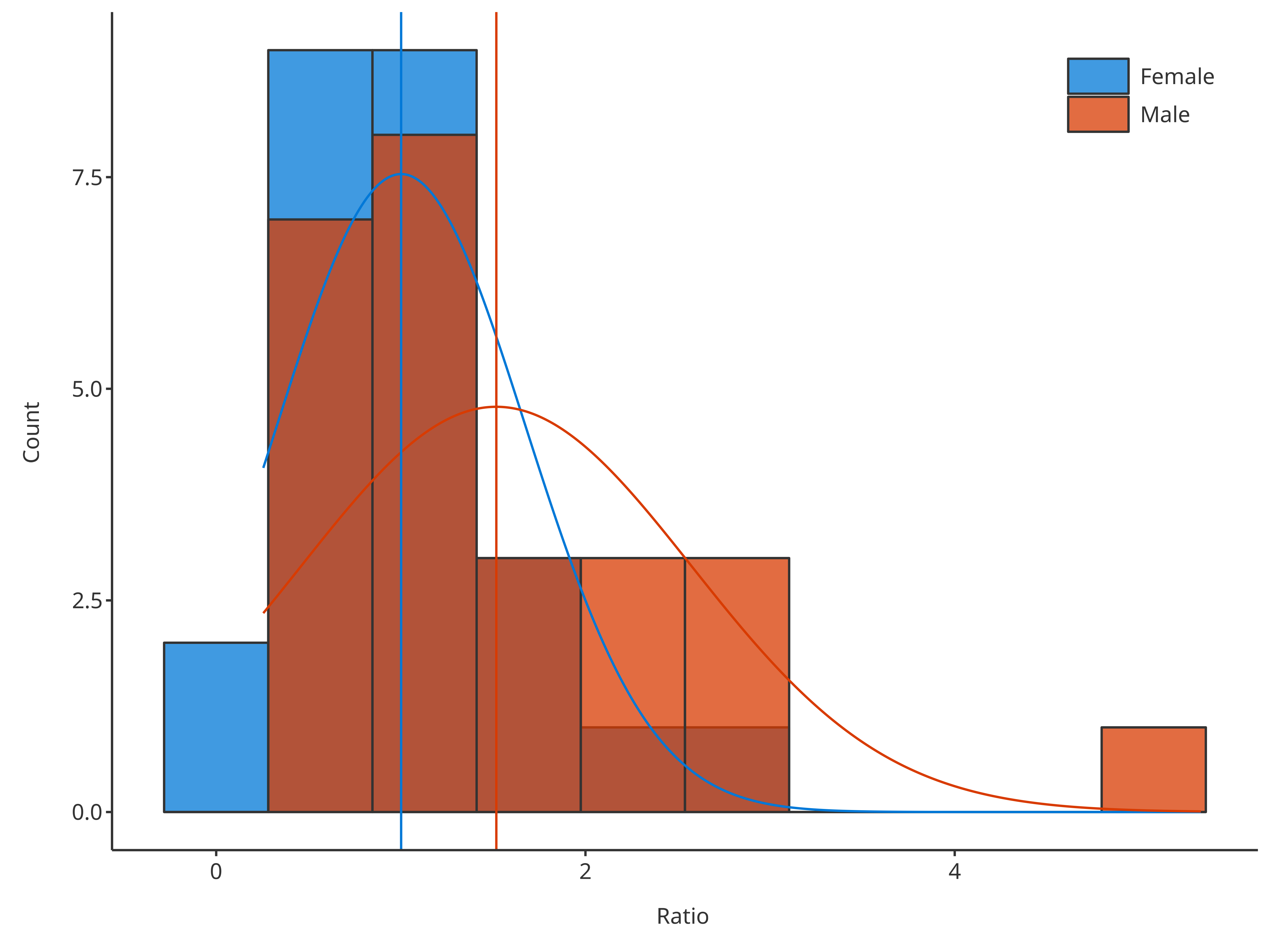
With option stack, it is also possible to get the distribution of the sum only while splitting the content of the bars.

# Create HistogramDataMapping object split by gender
histoMapping <- HistogramDataMapping$new(
  x = "Ratio",
  fill = "Sex"
)

# Plot normal distribution of sum but bars are split by gender
plotHistogram(
  data = histData,
  dataMapping = histoMapping,
  distribution = "normal",
  stack = TRUE
)

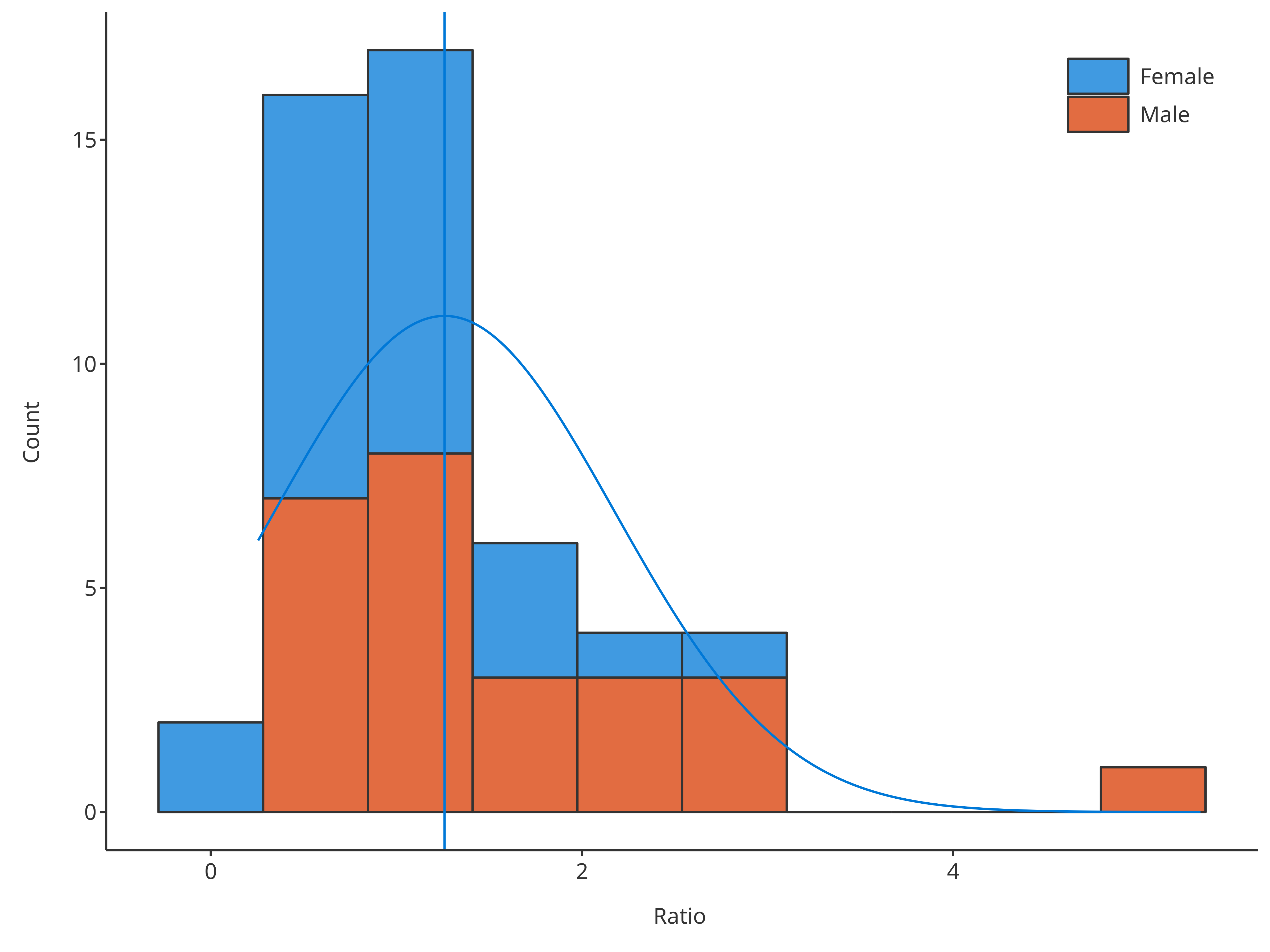
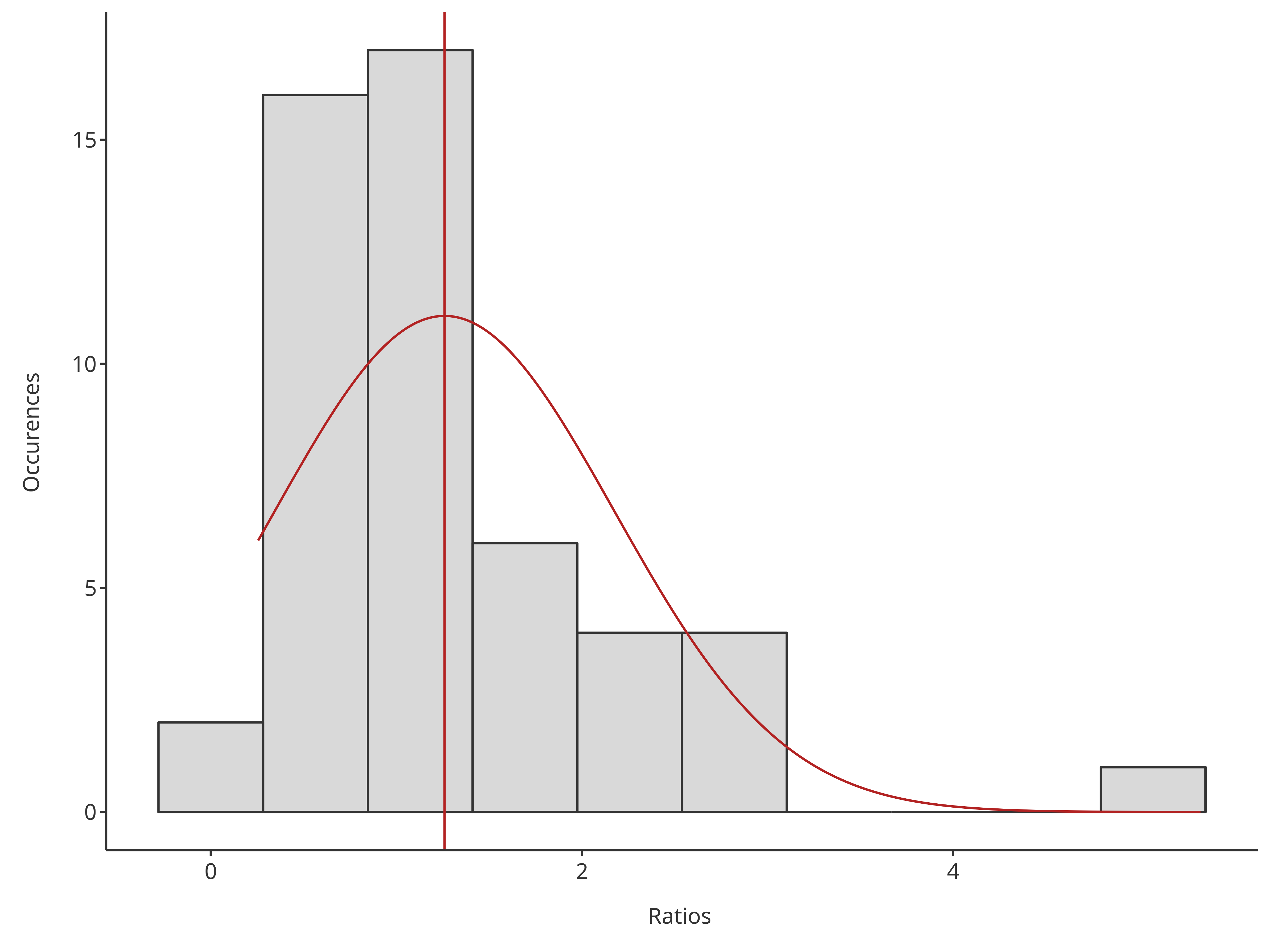
The HistogramPlotConfiguration objects can be used to tune the final plot aesthetics.

histoConfiguration <- HistogramPlotConfiguration$new(
  xlabel = "Ratios",
  ylabel = "Occurences"
)
histoConfiguration$ribbons$fill <- "grey80"
histoConfiguration$lines$color <- "firebrick"

# Plot normal distribution of sum but bars are split by gender
plotHistogram(
  x = histData$Ratio,
  plotConfiguration = histoConfiguration,
  distribution = "normal"
)