Time profiles and Residuals task • ospsuite.reportingengine

require(ospsuite.reportingengine)
#> Loading required package: ospsuite.reportingengine
#> Loading required package: ospsuite
#> Loading required package: rClr
#> Loading the dynamic library for Microsoft .NET runtime...
#> Loaded Common Language Runtime version 4.0.30319.42000
#> Loading required package: tlf

This vignette focuses on time profiles and residuals plots (also called goodness of fit plots) generated using either mean model or population workflows.

Overview

The time profiles and residuals task first aims at generating time profile plots of specified simulation paths. The task can account for observed data, in which case residuals are calculated and plotted. For population workflows, aggregation functions are used, by default mean, median, 5th and 95th percentiles are computed and plotted in the time profiles.

Inputs

Results obtained from the simulate task and stored as csv files within the subdirectory SimulationResults from the workflowFolder directory are required in order to perform the goodness of fit (plotTimeProfilesAndResiduals) task. As a consequence, if the workflow output folder does not include the appropriate simulations, the task simulate needs to be active.

The objects SimulationSet (or PopulationSimulationSet for population workflows) and Output define which and how the simulated and, if available, observed data will be plotted.

Outputs

The time profiles and residuals task generates for each simulation set plots of:

the simulated time profile
- in linear and logarithmic scale
- if available with data
- for total simulated time range.

Multiple applications

For simulations with multiple applications, up to 6 time profile plots can be generated corresponding to simulated time profiles in linear and logarithmic scale for:

the total simulated time range
the time range of the first application
the time range of the last application

The input applicationRanges from SimulationSet objects can be used to select which ranges to include in the evaluation.

Residuals

If observed data are available in the range selected in the output definition and selected in dataSelection, they will be added to the time profile plots.

Furthermore, residuals will be calculated according to the residual scale defined by the Output objects included within the simulation sets and 6 additional plots will be created figures:

Predicted vs observed in linear scale
Predicted vs observed in log scale
Residuals vs time
Residuals vs simulated output
Histogram of residuals
qq-plot of residuals

The residual scale corresponds to one element from the enum ResidualScales:

ResidualScales
#> $Linear
#> [1] "Linear"
#> 
#> $Logarithmic
#> [1] "Logarithmic"

The default uses “Logarithmic” and calculate residuals as: \(Residuals=log(Observed)-log(Simulated)\)

If the option “Linear” is used instead, the residuals are calculated as: \(Residuals=Observed-Simulated\)

A histogram and a qq-plot of residuals across all the simulation sets will also be added at the end of the analysis.

For population workflows, residuals are calculated from the aggregation of the Simulated output. By default, \(median(Simulated)\) is used instead of \(Simulated\). It is possible to modify this aggregation function by updating the fields of the object AggregationConfiguration.

Template examples

The following sections will introduce template scripts including goodness of fit tasks as well as their associated reports. Table 1 shows the features tested in each template script.

Table 1: Features tested by each template script
Example	Workflow	Simulation Sets	Outputs	Observed Data
1	Mean model	1	1	No
2	Mean model	1	1	Yes
3	Mean model	1	1	Yes
4	Mean model	1	2	Yes
5	Mean model	2	1	Yes
6	Population model	1	1	No
7	Population model	1	1	Yes

Example 1

Example 1 shows one of the simplest workflows including a goodness of fit. In this example, only a simulation time profile is performed since there is no observed data. Furthermore, only one simulation set and one output are requested.

Code

# Get the pkml simulation file: "MiniModel2.pkml"
simulationFile <- system.file("extdata", "MiniModel2.pkml",
  package = "ospsuite.reportingengine"
)

# Define the input parameters
outputA <- Output$new(
  path = "Organism|A|Concentration in container",
  displayName = "Concentration of A",
  displayUnit = "nmol/ml"
)

setA <- SimulationSet$new(
  simulationSetName = "A",
  simulationFile = simulationFile,
  outputs = outputA
)

# Create the workflow instance
workflow1 <-
  MeanModelWorkflow$new(
    simulationSets = setA,
    workflowFolder = "Example-1"
  )
#> 10/03/2023 - 15:23:18
#>  [32m [1mi Info   [22m [39mReporting Engine Information:
#>  Date: 10/03/2023 - 15:23:18
#>  User Information:
#>  Computer Name: WDEC030076
#>  User: ZTSOJ
#>  Login: ZTSOJ
#>  System is NOT validated
#>  System versions:
#>  R version: R version 4.2.2 (2022-10-31 ucrt)
#>  OSP Suite Package version: 11.1.198
#>  OSP Reporting Engine version: 2.1.244
#>  tlf version: 1.5.125

# Set the workflow tasks to be run
workflow1$activateTasks(c("simulate", "plotTimeProfilesAndResiduals"))

# Run the workflow
workflow1$runWorkflow()
#> 10/03/2023 - 15:23:18
#>  [32m [1mi Info   [22m [39mStarting run of  [36m [1m [3mMean Model Workflow [23m [22m [39m
#> 10/03/2023 - 15:23:18
#>  [32m [1mi Info   [22m [39mStarting run of  [36m [1m [3mSimulation task [23m [22m [39m
#> 10/03/2023 - 15:23:19
#>  [32m [1mi Info   [22m [39mSplitting simulations for parallel run: [36m [1m [3m1 [23m [22m [39m simulations split into  [36m [1m [3m1 [23m [22m [39m subsets
#> 10/03/2023 - 15:23:19
#>  [32m [1mi Info   [22m [39mStarting run of  [36m [1m [3msubset simulations [23m [22m [39m
#> 
  |                                                                            
  |                                                                      |   0%
  |                                                                            
  |======================================================================| 100%
#> 10/03/2023 - 15:23:19
#>  [32m [1mi Info   [22m [39m [36m [1m [3mSimulation task [23m [22m [39m completed in 0 min
#> 10/03/2023 - 15:23:19
#>  [32m [1mi Info   [22m [39mStarting run of  [36m [1m [3mPlot Time profiles and Residuals task [23m [22m [39m
#> 10/03/2023 - 15:23:19
#>  [32m [1mi Info   [22m [39mStarting run of  [36m [1m [3mPlot Time profiles and Residuals task [23m [22m [39m for  [36m [1m [3mA [23m [22m [39m
#> 10/03/2023 - 15:23:23
#>  [32m [1mi Info   [22m [39m [36m [1m [3mPlot Time profiles and Residuals task [23m [22m [39m completed in 0.1 min
#> Executing: pandoc --self-contained --wrap=none --toc --from=markdown+tex_math_dollars+superscript+subscript+raw_attribute --reference-doc="C:/Users/ztsoj/AppData/Local/Temp/RtmpwxXS6L/temp_libpath298c4a21481f/ospsuite.reportingengine/extdata/reference.docx" --resource-path="Example-1" -t docx -o "Example-1/Report-word.docx" "Example-1/Report-word.md"
#> 10/03/2023 - 15:23:25
#>  [32m [1mi Info   [22m [39m [36m [1m [3mMean Model Workflow [23m [22m [39m completed in 0.1 min

The output report for Example 1 is shown below. There are only 2 figures in the report (linear and log scales) showing the time profile of the output path ‘Organism|A|Concentration in container’ displayed as ‘Concentration of A’.

Report

Example 2

Example 2 shows a workflow that used the simulation results performed in Example 1. This example shows 3 new features:

The presence of observed data compared to the simulation
The use of results obtained from a previous workflow
The change of display unit without re-running the simulate task

Code

# Get the pkml simulation file: "MiniModel2.pkml"
simulationFile <- system.file("extdata", "MiniModel2.pkml",
  package = "ospsuite.reportingengine"
)

# Get the observation file and its dictionary
observationFile = system.file(
  "extdata", "SimpleData.nmdat",
  package = "ospsuite.reportingengine"
)
dictionaryFile = system.file(
  "extdata", "tpDictionary.csv",
  package = "ospsuite.reportingengine"
)
dataSource <- DataSource$new(
  dataFile = observationFile,
  metaDataFile = dictionaryFile
)

# Define the input parameters
outputA <- Output$new(
  path = "Organism|A|Concentration in container",
  displayName = "Simulated concentration of A",
  displayUnit = "µmol/ml",
  dataSelection = "MDV==0",
  dataDisplayName = "Observed concentration of A"
)

setA <- SimulationSet$new(
  simulationSetName = "A",
  simulationFile = simulationFile,
  outputs = outputA,
  dataSource = dataSource
)

# Create the workflow instance
workflow2 <-
  MeanModelWorkflow$new(
    simulationSets = setA,
    workflowFolder = "Example-1"
  )
#> 10/03/2023 - 15:23:32
#> i Info  Reporting Engine Information:
#>  Date: 10/03/2023 - 15:23:32
#>  User Information:
#>  Computer Name: WDEC030076
#>  User: ZTSOJ
#>  Login: ZTSOJ
#>  System is NOT validated
#>  System versions:
#>  R version: R version 4.2.2 (2022-10-31 ucrt)
#>  OSP Suite Package version: 11.1.198
#>  OSP Reporting Engine version: 2.1.244
#>  tlf version: 1.5.125

# Set the workflow tasks to be run
workflow2$activateTasks("plotTimeProfilesAndResiduals")
workflow2$inactivateTasks("simulate")

# Run the workflow
workflow2$runWorkflow()
#> 10/03/2023 - 15:23:32
#> i Info  Starting run of Mean Model Workflow
#> 10/03/2023 - 15:23:32
#> i Info  Starting run of Plot Time profiles and Residuals task
#> 10/03/2023 - 15:23:32
#> i Info  Starting run of Plot Time profiles and Residuals task for A
#> 10/03/2023 - 15:23:45
#> i Info  Plot Time profiles and Residuals task completed in 0.2 min
#> Executing: pandoc --self-contained --wrap=none --toc --from=markdown+tex_math_dollars+superscript+subscript+raw_attribute --reference-doc="C:/Users/ztsoj/AppData/Local/Temp/RtmpwxXS6L/temp_libpath298c4a21481f/ospsuite.reportingengine/extdata/reference.docx" --resource-path="Example-1" -t docx -o "Example-1/Report-word.docx" "Example-1/Report-word.md"
#> 10/03/2023 - 15:23:48
#> i Info  Mean Model Workflow completed in 0.3 min

It can be seen from the run results that the task simulate was not run.

In this example, the content of the observed data file and its dictionary are respectively described Table 2 and 3.

Table 2: Observed data content
ID	STUD	SID	TIME	TAD	DV	CMT	MDV	AMT	WGHT	HGHT	SEX	AGE	LOQ
1	9999	1	0	0	0.00000	2	1	450	82	160	1	32	0.001
2	9999	1	2	2	0.00120	1	0	0	82	160	1	32	0.001
3	9999	1	4	4	0.00142	1	0	0	82	160	1	32	0.001
4	9999	1	6	6	0.00163	1	0	0	82	160	1	32	0.001
5	9999	1	8	8	0.00269	1	0	0	82	160	1	32	0.001

Table 3: Dictionary content
ID	type	datasetColumn	datasetUnit	reportName	pathID	comment
sid	identifier	SID
stud	identifier	STUD
time	timeprofile	TIME	h
dv	timeprofile	DV	mg/ml
tad	timeprofile	TAD	h
age	covariate	AGE	year(s)	Age	Organism\|Age
wght	covariate	WGHT	kg	Body weight	Organism\|Weight
hght	covariate	HGHT	cm	Height	Organism\|Height
bmi	covariate	BMI	kg/m2	BMI	Organism\|BMI
gender	covariate	SEX		SEX	Gender	Make sure 1=male 2= female

The output report for Example 2 is shown below. There are now many more figures in the report showing not only time profiles in µmol/ml instead of nmol/ml but also residuals.

Report

Example 3

In example 3, the dictionary is changed and indicates that the lower limit of quantitation (LLOQ) is included in the observed data. Like the previous example, there is no need to re-run the simulate task.

Code

# Get the pkml simulation file: "MiniModel2.pkml"
simulationFile <- system.file("extdata", "MiniModel2.pkml",
  package = "ospsuite.reportingengine"
)

# Get the observation file and its dictionary
dataSource <- DataSource$new(
  dataFile = observationFile,
  metaDataFile = system.file(
    "extdata", "tpDictionaryLoq.csv",
    package = "ospsuite.reportingengine"
    )
)

# Define the input parameters
outputA <- Output$new(
  path = "Organism|A|Concentration in container",
  displayName = "Simulated concentration of A",
  displayUnit = "µmol/ml",
  dataSelection = "MDV==0",
  dataDisplayName = "Observed concentration of A"
)

setA <- SimulationSet$new(
  simulationSetName = "A",
  simulationFile = simulationFile,
  outputs = outputA,
  dataSource = dataSource
)

# Create the workflow instance
workflow3 <-
  MeanModelWorkflow$new(
    simulationSets = setA,
    workflowFolder = "Example-1"
  )
#> 10/03/2023 - 15:23:58
#> i Info  Reporting Engine Information:
#>  Date: 10/03/2023 - 15:23:58
#>  User Information:
#>  Computer Name: WDEC030076
#>  User: ZTSOJ
#>  Login: ZTSOJ
#>  System is NOT validated
#>  System versions:
#>  R version: R version 4.2.2 (2022-10-31 ucrt)
#>  OSP Suite Package version: 11.1.198
#>  OSP Reporting Engine version: 2.1.244
#>  tlf version: 1.5.125

# Set the workflow tasks to be run
workflow3$activateTasks("plotTimeProfilesAndResiduals")
workflow3$inactivateTasks("simulate")

# Run the workflow
workflow3$runWorkflow()
#> 10/03/2023 - 15:23:59
#> i Info  Starting run of Mean Model Workflow
#> 10/03/2023 - 15:23:59
#> i Info  Starting run of Plot Time profiles and Residuals task
#> 10/03/2023 - 15:23:59
#> i Info  Starting run of Plot Time profiles and Residuals task for A
#> 10/03/2023 - 15:24:14
#> i Info  Plot Time profiles and Residuals task completed in 0.3 min
#> Executing: pandoc --self-contained --wrap=none --toc --from=markdown+tex_math_dollars+superscript+subscript+raw_attribute --reference-doc="C:/Users/ztsoj/AppData/Local/Temp/RtmpwxXS6L/temp_libpath298c4a21481f/ospsuite.reportingengine/extdata/reference.docx" --resource-path="Example-1" -t docx -o "Example-1/Report-word.docx" "Example-1/Report-word.md"
#> 10/03/2023 - 15:24:16
#> i Info  Mean Model Workflow completed in 0.3 min

The new dictionary content is described in Table 4.

Table 4: Dictionary content
ID	type	datasetColumn	datasetUnit	reportName	pathID	comment
sid	identifier	SID
stud	identifier	STUD
time	timeprofile	TIME	h
dv	timeprofile	DV	mg/ml
tad	timeprofile	TAD	h
age	covariate	AGE	year(s)	Age	Organism\|Age
wght	covariate	WGHT	kg	Body weight	Organism\|Weight
hght	covariate	HGHT	cm	Height	Organism\|Height
bmi	covariate	BMI	kg/m2	BMI	Organism\|BMI
gender	covariate	SEX		SEX	Gender	Make sure 1=male 2= female

The output report for Example 3 is shown below. The time profiles now indicate the LLOQ.

Report

Example 4

In example 4, the simulation set now includes 2 output paths. Output path Organism|A|Concentration in container has observed data to be compared to whereas output path Organism|B|Concentration in container does not. Since output path Organism|B|Concentration in container was not requested by the examples 1, 2 and 3, it is not included in the simulation results. As a consequence, the simulate task needs to be re-run.

Code

# Get the pkml simulation file: "MiniModel2.pkml"
simulationFile <- system.file("extdata", "MiniModel2.pkml",
  package = "ospsuite.reportingengine"
)

# Get the observation file and its dictionary
dataSource <- DataSource$new(
  dataFile = observationFile,
  metaDataFile = dictionaryFile
)

# Define the input parameters
outputA <- Output$new(
  path = "Organism|A|Concentration in container",
  displayName = "Simulated concentration of A",
  displayUnit = "µmol/ml",
  dataSelection = "MDV==0",
  dataDisplayName = "Observed concentration of A"
)
outputB <- Output$new(
  path = "Organism|B|Concentration in container",
  displayName = "Simulated concentration of B",
  displayUnit = "µmol/ml"
)

setAB <- SimulationSet$new(
  simulationSetName = "A and B",
  simulationFile = simulationFile,
  outputs = c(outputA, outputB),
  dataSource = dataSource
)

# Create the workflow instance
workflow4 <-
  MeanModelWorkflow$new(
    simulationSets = setAB,
    workflowFolder = "Example-4"
  )
#> 10/03/2023 - 15:24:24
#>  [32m [1mi Info   [22m [39mReporting Engine Information:
#>  Date: 10/03/2023 - 15:24:24
#>  User Information:
#>  Computer Name: WDEC030076
#>  User: ZTSOJ
#>  Login: ZTSOJ
#>  System is NOT validated
#>  System versions:
#>  R version: R version 4.2.2 (2022-10-31 ucrt)
#>  OSP Suite Package version: 11.1.198
#>  OSP Reporting Engine version: 2.1.244
#>  tlf version: 1.5.125

# Set the workflow tasks to be run
workflow4$activateTasks(c("simulate", "plotTimeProfilesAndResiduals"))

# Run the workflow
workflow4$runWorkflow()
#> 10/03/2023 - 15:24:24
#>  [32m [1mi Info   [22m [39mStarting run of  [36m [1m [3mMean Model Workflow [23m [22m [39m
#> 10/03/2023 - 15:24:24
#>  [32m [1mi Info   [22m [39mStarting run of  [36m [1m [3mSimulation task [23m [22m [39m
#> 10/03/2023 - 15:24:25
#>  [32m [1mi Info   [22m [39mSplitting simulations for parallel run: [36m [1m [3m1 [23m [22m [39m simulations split into  [36m [1m [3m1 [23m [22m [39m subsets
#> 10/03/2023 - 15:24:25
#>  [32m [1mi Info   [22m [39mStarting run of  [36m [1m [3msubset simulations [23m [22m [39m
#> 
  |                                                                            
  |                                                                      |   0%
  |                                                                            
  |======================================================================| 100%
#> 10/03/2023 - 15:24:25
#>  [32m [1mi Info   [22m [39m [36m [1m [3mSimulation task [23m [22m [39m completed in 0 min
#> 10/03/2023 - 15:24:25
#>  [32m [1mi Info   [22m [39mStarting run of  [36m [1m [3mPlot Time profiles and Residuals task [23m [22m [39m
#> 10/03/2023 - 15:24:25
#>  [32m [1mi Info   [22m [39mStarting run of  [36m [1m [3mPlot Time profiles and Residuals task [23m [22m [39m for  [36m [1m [3mA and B [23m [22m [39m
#> 10/03/2023 - 15:24:37
#>  [32m [1mi Info   [22m [39m [36m [1m [3mPlot Time profiles and Residuals task [23m [22m [39m completed in 0.2 min
#> Executing: pandoc --self-contained --wrap=none --toc --from=markdown+tex_math_dollars+superscript+subscript+raw_attribute --reference-doc="C:/Users/ztsoj/AppData/Local/Temp/RtmpwxXS6L/temp_libpath298c4a21481f/ospsuite.reportingengine/extdata/reference.docx" --resource-path="Example-4" -t docx -o "Example-4/Report-word.docx" "Example-4/Report-word.md"
#> 10/03/2023 - 15:24:39
#>  [32m [1mi Info   [22m [39m [36m [1m [3mMean Model Workflow [23m [22m [39m completed in 0.2 min

The output report for Example 4 is shown below.

Report

Example 5

In example 5, there are 2 simulation sets, each one includes one output path. Simulation set A includes output path Organism|A|Concentration in container and has observed data. Simulation set B includes output path Organism|B|Concentration in container and has no observed data. The simulate task needs to be re-run also in this case since the simulation results are saved in files that use the simulation set names.

Code

# Get the pkml simulation file: "MiniModel1.pkml"
simulationFileA <- system.file("extdata", "MiniModel1.pkml",
  package = "ospsuite.reportingengine"
)

# Get the pkml simulation file: "MiniModel2.pkml"
simulationFileB <- system.file("extdata", "MiniModel2.pkml",
  package = "ospsuite.reportingengine"
)

# Get the observation file and its dictionary
dataSource <- DataSource$new(
  dataFile = observationFile,
  metaDataFile = dictionaryFile
)

# Define the input parameters
outputA <- Output$new(
  path = "Organism|A|Concentration in container",
  displayName = "Simulated concentration of A",
  displayUnit = "µmol/ml",
  dataSelection = "MDV==0",
  dataDisplayName = "Observed concentration of A"
)
outputB <- Output$new(
  path = "Organism|B|Concentration in container",
  displayName = "Simulated concentration of B",
  displayUnit = "µmol/ml"
)

setA <- SimulationSet$new(
  simulationSetName = "A",
  simulationFile = simulationFileA,
  outputs = outputA,
  dataSource = dataSource
)
setB <- SimulationSet$new(
  simulationSetName = "B",
  simulationFile = simulationFileB,
  outputs = outputB
)

# Create the workflow instance
workflow5 <-
  MeanModelWorkflow$new(
    simulationSets = c(setA, setB),
    workflowFolder = "Example-5"
  )
#> 10/03/2023 - 15:24:47
#>  [32m [1mi Info   [22m [39mReporting Engine Information:
#>  Date: 10/03/2023 - 15:24:47
#>  User Information:
#>  Computer Name: WDEC030076
#>  User: ZTSOJ
#>  Login: ZTSOJ
#>  System is NOT validated
#>  System versions:
#>  R version: R version 4.2.2 (2022-10-31 ucrt)
#>  OSP Suite Package version: 11.1.198
#>  OSP Reporting Engine version: 2.1.244
#>  tlf version: 1.5.125

# Set the workflow tasks to be run
workflow5$activateTasks(c("simulate", "plotTimeProfilesAndResiduals"))

# Run the workflow
workflow5$runWorkflow()
#> 10/03/2023 - 15:24:47
#>  [32m [1mi Info   [22m [39mStarting run of  [36m [1m [3mMean Model Workflow [23m [22m [39m
#> 10/03/2023 - 15:24:47
#>  [32m [1mi Info   [22m [39mStarting run of  [36m [1m [3mSimulation task [23m [22m [39m
#> 10/03/2023 - 15:24:47
#>  [32m [1mi Info   [22m [39mSplitting simulations for parallel run: [36m [1m [3m2 [23m [22m [39m simulations split into  [36m [1m [3m1 [23m [22m [39m subsets
#> 10/03/2023 - 15:24:47
#>  [32m [1mi Info   [22m [39mStarting run of  [36m [1m [3msubset simulations [23m [22m [39m
#> 
  |                                                                            
  |                                                                      |   0%
  |                                                                            
  |======================================================================| 100%
#> 10/03/2023 - 15:24:48
#>  [32m [1mi Info   [22m [39m [36m [1m [3mSimulation task [23m [22m [39m completed in 0 min
#> 10/03/2023 - 15:24:48
#>  [32m [1mi Info   [22m [39mStarting run of  [36m [1m [3mPlot Time profiles and Residuals task [23m [22m [39m
#> 10/03/2023 - 15:24:48
#>  [32m [1mi Info   [22m [39mStarting run of  [36m [1m [3mPlot Time profiles and Residuals task [23m [22m [39m for  [36m [1m [3mA [23m [22m [39m
#> 10/03/2023 - 15:24:59
#>  [32m [1mi Info   [22m [39mStarting run of  [36m [1m [3mPlot Time profiles and Residuals task [23m [22m [39m for  [36m [1m [3mB [23m [22m [39m
#> 10/03/2023 - 15:25:10
#>  [32m [1mi Info   [22m [39m [36m [1m [3mPlot Time profiles and Residuals task [23m [22m [39m completed in 0.4 min
#> Executing: pandoc --self-contained --wrap=none --toc --from=markdown+tex_math_dollars+superscript+subscript+raw_attribute --reference-doc="C:/Users/ztsoj/AppData/Local/Temp/RtmpwxXS6L/temp_libpath298c4a21481f/ospsuite.reportingengine/extdata/reference.docx" --resource-path="Example-5" -t docx -o "Example-5/Report-word.docx" "Example-5/Report-word.md"
#> 10/03/2023 - 15:25:12
#>  [32m [1mi Info   [22m [39m [36m [1m [3mMean Model Workflow [23m [22m [39m completed in 0.4 min

The output report for Example 5 is shown below.

Report

Example 6

Example 6 shows a goodness of fit for a population workflow. In this example, there is no observed data, only one simulation set and one output are requested.

Code

# Get the pkml simulation file: "MiniModel2.pkml"
simulationFile <- system.file("extdata", "MiniModel2.pkml",
  package = "ospsuite.reportingengine"
)

populationFile <- system.file("extdata", "Pop500_p1p2p3.csv",
  package = "ospsuite.reportingengine"
)

# Define the input parameters
outputA <- Output$new(
  path = "Organism|A|Concentration in container",
  displayName = "Concentration of A",
  displayUnit = "µmol/ml"
)

setA <- PopulationSimulationSet$new(
  simulationSetName = "A",
  simulationFile = simulationFile,
  populationFile = populationFile,
  outputs = outputA
)

# Create the workflow instance
workflow6 <-
  PopulationWorkflow$new(
    workflowType = PopulationWorkflowTypes$parallelComparison,
    simulationSets = setA,
    workflowFolder = "Example-6"
  )
#> 10/03/2023 - 15:25:22
#> i Info  Reporting Engine Information:
#>  Date: 10/03/2023 - 15:25:22
#>  User Information:
#>  Computer Name: WDEC030076
#>  User: ZTSOJ
#>  Login: ZTSOJ
#>  System is NOT validated
#>  System versions:
#>  R version: R version 4.2.2 (2022-10-31 ucrt)
#>  OSP Suite Package version: 11.1.198
#>  OSP Reporting Engine version: 2.1.244
#>  tlf version: 1.5.125

# Set the workflow tasks to be run
workflow6$activateTasks(c("simulate", "plotTimeProfilesAndResiduals"))

# Run the workflow
workflow6$runWorkflow()
#> 10/03/2023 - 15:25:22
#> i Info  Starting run of Population Workflow for parallelComparison
#> 10/03/2023 - 15:25:22
#> i Info  Starting run of Simulation task
#> 10/03/2023 - 15:25:23
#> i Info  Simulation task completed in 0 min
#> 10/03/2023 - 15:25:23
#> i Info  Starting run of Plot Time profiles and Residuals task
#> 10/03/2023 - 15:25:23
#> i Info  Starting run of Plot Time profiles and Residuals task for A
#> 10/03/2023 - 15:25:28
#> i Info  Plot Time profiles and Residuals task completed in 0.1 min
#> Executing: pandoc --self-contained --wrap=none --toc --from=markdown+tex_math_dollars+superscript+subscript+raw_attribute --reference-doc="C:/Users/ztsoj/AppData/Local/Temp/RtmpwxXS6L/temp_libpath298c4a21481f/ospsuite.reportingengine/extdata/reference.docx" --resource-path="Example-6" -t docx -o "Example-6/Report-word.docx" "Example-6/Report-word.md"
#> 10/03/2023 - 15:25:30
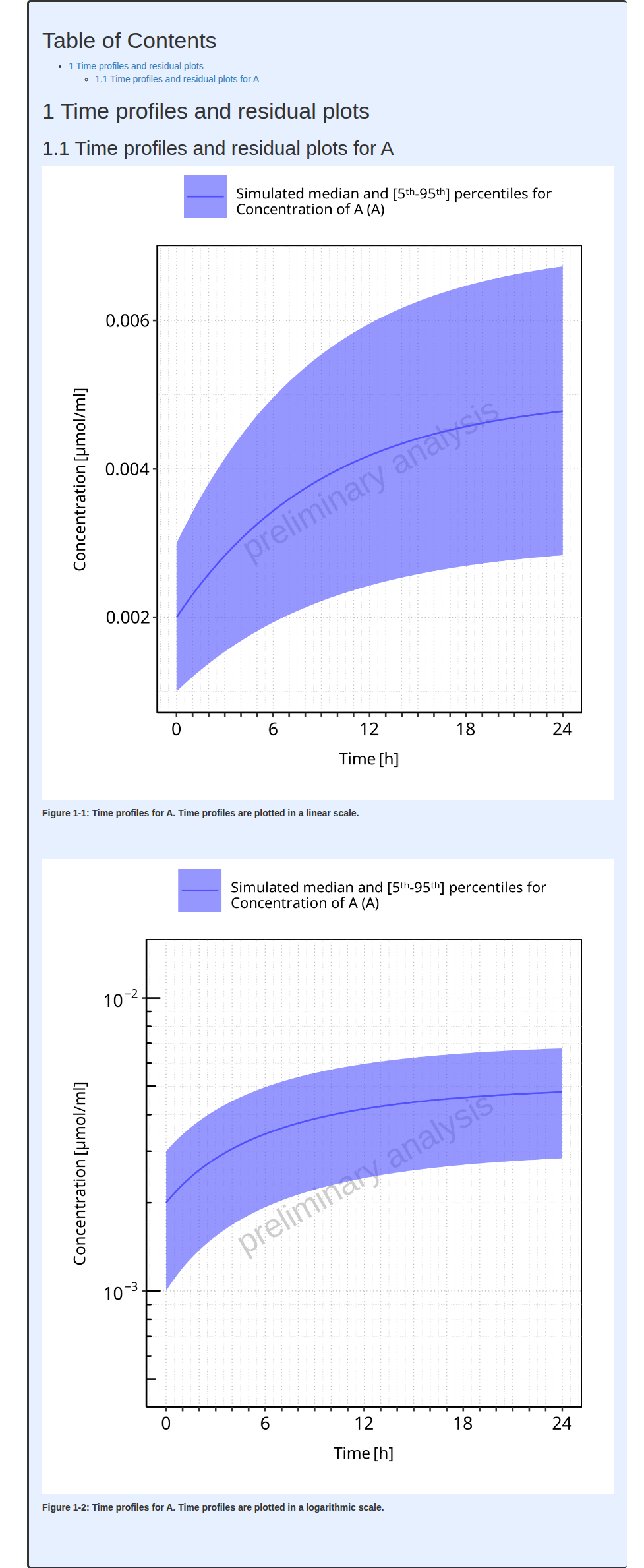
#> i Info  Population Workflow for parallelComparison completed in 0.1 min

The output report for Example 6 is shown below. The 2 figures of the report (linear and log scales) include median, mean 5th and 95th percentiles of the population.

Report

Example 7

Example 7 add observed data to the previous workflow.

Code

# Get the pkml simulation file: "MiniModel2.pkml"
simulationFile <- system.file("extdata", "MiniModel2.pkml",
  package = "ospsuite.reportingengine"
)
populationFile <- system.file("extdata", "Pop500_p1p2p3.csv",
  package = "ospsuite.reportingengine"
)

# Get the observation file and its dictionary
dataSource <- DataSource$new(
  dataFile = observationFile,
  metaDataFile = dictionaryFile
)

# Define the input parameters
outputA <- Output$new(
  path = "Organism|A|Concentration in container",
  displayName = "Simulated concentration of A",
  displayUnit = "µmol/ml",
  dataSelection = "MDV==0",
  dataDisplayName = "Observed concentration of A"
)

setA <- PopulationSimulationSet$new(
  simulationSetName = "A",
  simulationFile = simulationFile,
  populationFile = populationFile,
  outputs = outputA,
  dataSource = dataSource
)

# Create the workflow instance
workflow7 <-
  PopulationWorkflow$new(
    workflowType = PopulationWorkflowTypes$parallelComparison,
    simulationSets = setA,
    workflowFolder = "Example-6"
  )
#> 10/03/2023 - 15:25:36
#> i Info  Reporting Engine Information:
#>  Date: 10/03/2023 - 15:25:36
#>  User Information:
#>  Computer Name: WDEC030076
#>  User: ZTSOJ
#>  Login: ZTSOJ
#>  System is NOT validated
#>  System versions:
#>  R version: R version 4.2.2 (2022-10-31 ucrt)
#>  OSP Suite Package version: 11.1.198
#>  OSP Reporting Engine version: 2.1.244
#>  tlf version: 1.5.125

# Set the workflow tasks to be run
workflow7$activateTasks(StandardPlotTasks$plotTimeProfilesAndResiduals)
workflow7$inactivateTasks(StandardSimulationTasks$simulate)

# Run the workflow
workflow7$runWorkflow()
#> 10/03/2023 - 15:25:36
#> i Info  Starting run of Population Workflow for parallelComparison
#> 10/03/2023 - 15:25:36
#> i Info  Starting run of Plot Time profiles and Residuals task
#> 10/03/2023 - 15:25:36
#> i Info  Starting run of Plot Time profiles and Residuals task for A
#> 10/03/2023 - 15:25:50
#> i Info  Plot Time profiles and Residuals task completed in 0.2 min
#> Executing: pandoc --self-contained --wrap=none --toc --from=markdown+tex_math_dollars+superscript+subscript+raw_attribute --reference-doc="C:/Users/ztsoj/AppData/Local/Temp/RtmpwxXS6L/temp_libpath298c4a21481f/ospsuite.reportingengine/extdata/reference.docx" --resource-path="Example-6" -t docx -o "Example-6/Report-word.docx" "Example-6/Report-word.md"
#> 10/03/2023 - 15:25:53
#> i Info  Population Workflow for parallelComparison completed in 0.3 min

The output report for Example 7 is shown below. The residuals are calculated on the median simulated values.

Report