Box-Whisker Plots • ospsuite.plots

1. Introduction

This vignette documents and illustrates workflows for producing box-and-whisker plots using the ospsuite.plots library.

The function for plotting box-whiskers is plotBoxWhisker. Basic documentation of the function can be found using: ?plotBoxWhisker. The output of the function is a ggplot object.

1.1 Setup

This vignette uses the ospsuite.plots and tidyr libraries. We will use the default settings of ospsuite.plots (see vignette(“ospsuite.plots”, package = “ospsuite.plots”)) but will adjust the legend position and the alignment of the caption.

library(ospsuite.plots)
library(tidyr)

# Set Defaults
oldDefaults <- ospsuite.plots::setDefaults()

# Adjust default theme plot for prettier plots
theme_update(legend.position = "top")
theme_update(legend.direction = "horizontal")
theme_update(plot.caption = element_text(hjust = 1))

1.2 Example Data

This vignette uses a dataset provided by the package:

pkRatioData <- exampleDataCovariates %>%
  dplyr::filter(SetID == "DataSet1") %>%
  dplyr::select(-c("SetID", "gsd", "AgeBin")) %>%
  dplyr::mutate(Agegroup = cut(Age, breaks = c(0, 6, 12, 18, 60), include.lowest = TRUE, labels = c("infants", "school children", "adolescents", "adults")))

knitr::kable(head(pkRatioData), digits = 3, caption = "First rows of example data pkRatioData")

First rows of example data pkRatioData
ID	Age	Obs	Pred	Ratio	Sex	Country	SD	Agegroup
1	48	4.00	2.90	0.725	Male	Canada	0.693	adults
2	36	4.40	5.75	1.307	Male	Canada	0.188	adults
3	52	2.80	2.70	0.964	Male	Canada	0.984	adults
4	47	3.75	3.05	0.813	Male	Canada	0.591	adults
5	0	1.95	5.25	2.692	Male	Canada	0.443	infants
6	48	2.45	5.30	2.163	Male	Canada	0.072	adults

Metadata is a list that contains dimension and unit information for dataset columns. If available, axis labels are set by this information.

metaData <- attr(exampleDataCovariates, "metaData")
knitr::kable(metaData2DataFrame(metaData), digits = 2, caption = "List of meta data")

List of meta data
	Age	Obs	Pred	SD	Ratio
dimension	Age	Clearance	Clearance	Clearance	Ratio
unit	yrs	dL/h/kg	dL/h/kg	dL/h/kg

2. Examples

2.1 Examples for Aggregation of Categorical Data

2.1.1 Minimal Example

Age (mapped to y) is aggregated.

plotBoxWhisker(data = pkRatioData, mapping = aes(y = Age), metaData = metaData)
#> Warning in mappedData$doAdjustmentsWithMetaData(originalmapping = mapping, : No
#> metaData available for x-axis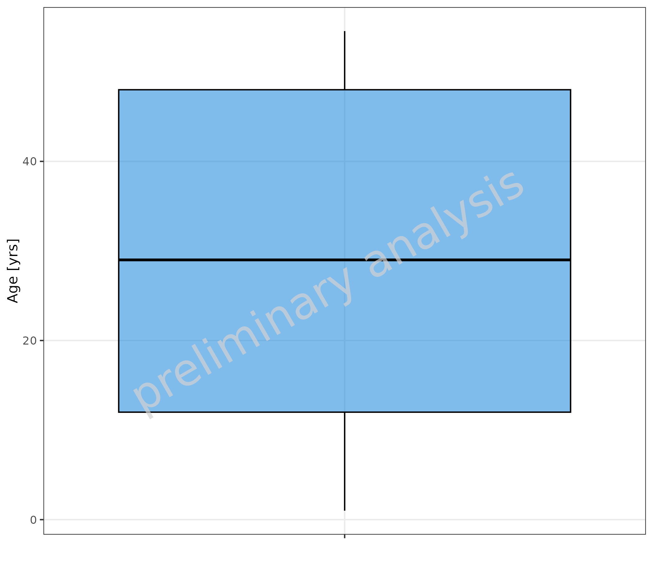

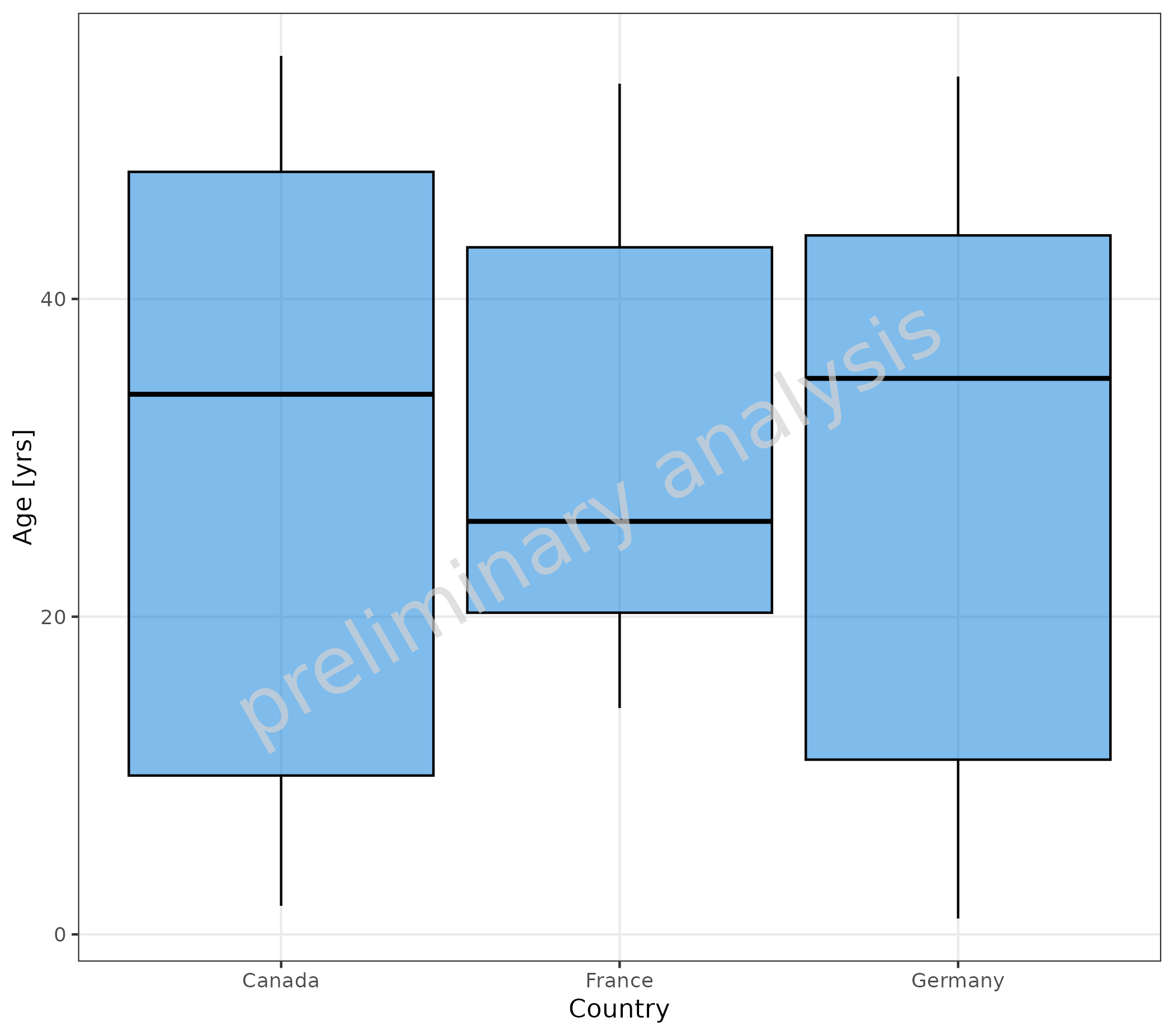
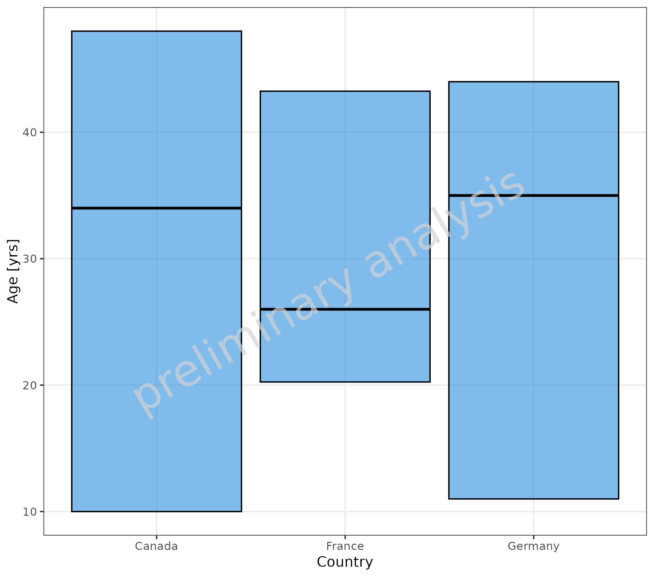
Box plot showing age distribution aggregated across all data. The plot displays quartiles with median line, showing the overall age range distribution.

2.1.2 Stratification on X-axis

Age (mapped to y) is aggregated for different countries (mapped to x).

plotBoxWhisker(
  mapping = aes(
    x = Country,
    y = Age
  ),
  data = pkRatioData,
  metaData = metaData
)

Box plots showing age distribution stratified by country. Separate box plots are displayed for each country on the x-axis, allowing comparison of age distributions between countries.

2.1.3 Stratification by Color

Age (mapped to y) is aggregated for different countries (mapped to fill).

plotBoxWhisker(
  mapping = aes(
    fill = Country,
    y = Age
  ),
  data = pkRatioData,
  metaData = metaData
)
#> Warning in mappedData$doAdjustmentsWithMetaData(originalmapping = mapping, : No
#> metaData available for x-axis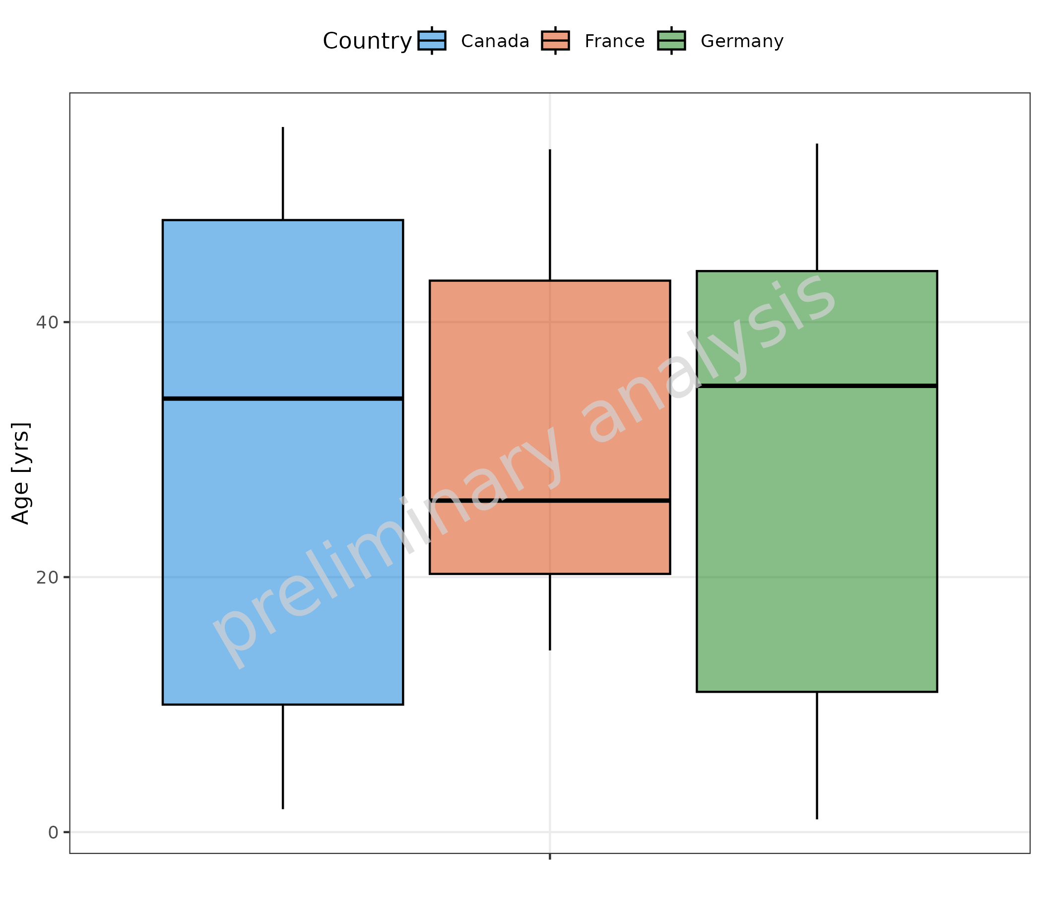

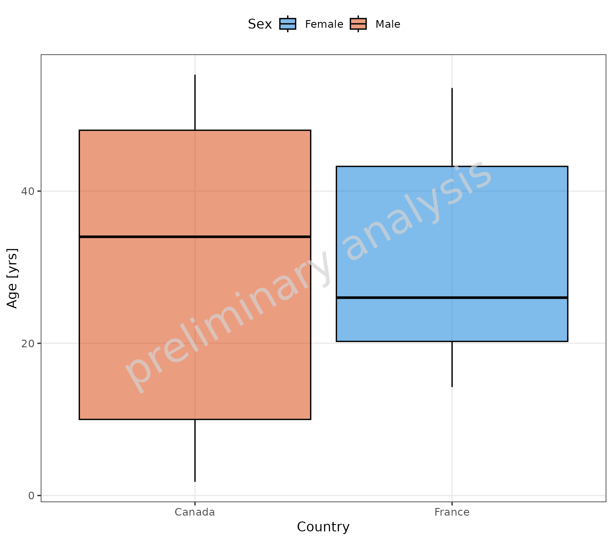
Box plot showing age distribution stratified by country using color coding. Different countries are represented by different fill colors in a single grouped box plot.

2.1.4 Stratification by Color and on X-axis

Age (mapped to y) is aggregated for different countries (mapped to x) and Sex (mapped to groupby). groupby is an additional aesthetic of ospsuite.plots that works together with the variable groupAesthetics. For the function plotBoxWhisker(), groupAesthetics is not settable and is fixed to fill.

plotBoxWhisker(
  mapping = aes(
    x = Country,
    y = Age,
    groupby = Sex
  ),
  data = pkRatioData,
  metaData = metaData
)

Box plots showing age distribution stratified by both country (x-axis) and sex (color/grouping). The plot displays separate box plots for each country, with different colors representing sex within each country.

2.1.5 Stratification by Column Combination

Below, groupby is mapped to a combination of the columns “Sex” and “Country”:

plotBoxWhisker(
  mapping = aes(
    y = Age,
    groupby = interaction(Country, Sex, sep = "-")
  ),
  data = pkRatioData,
  metaData = metaData
) + theme(legend.title = element_blank())
#> Warning in mappedData$doAdjustmentsWithMetaData(originalmapping = mapping, : No
#> metaData available for x-axis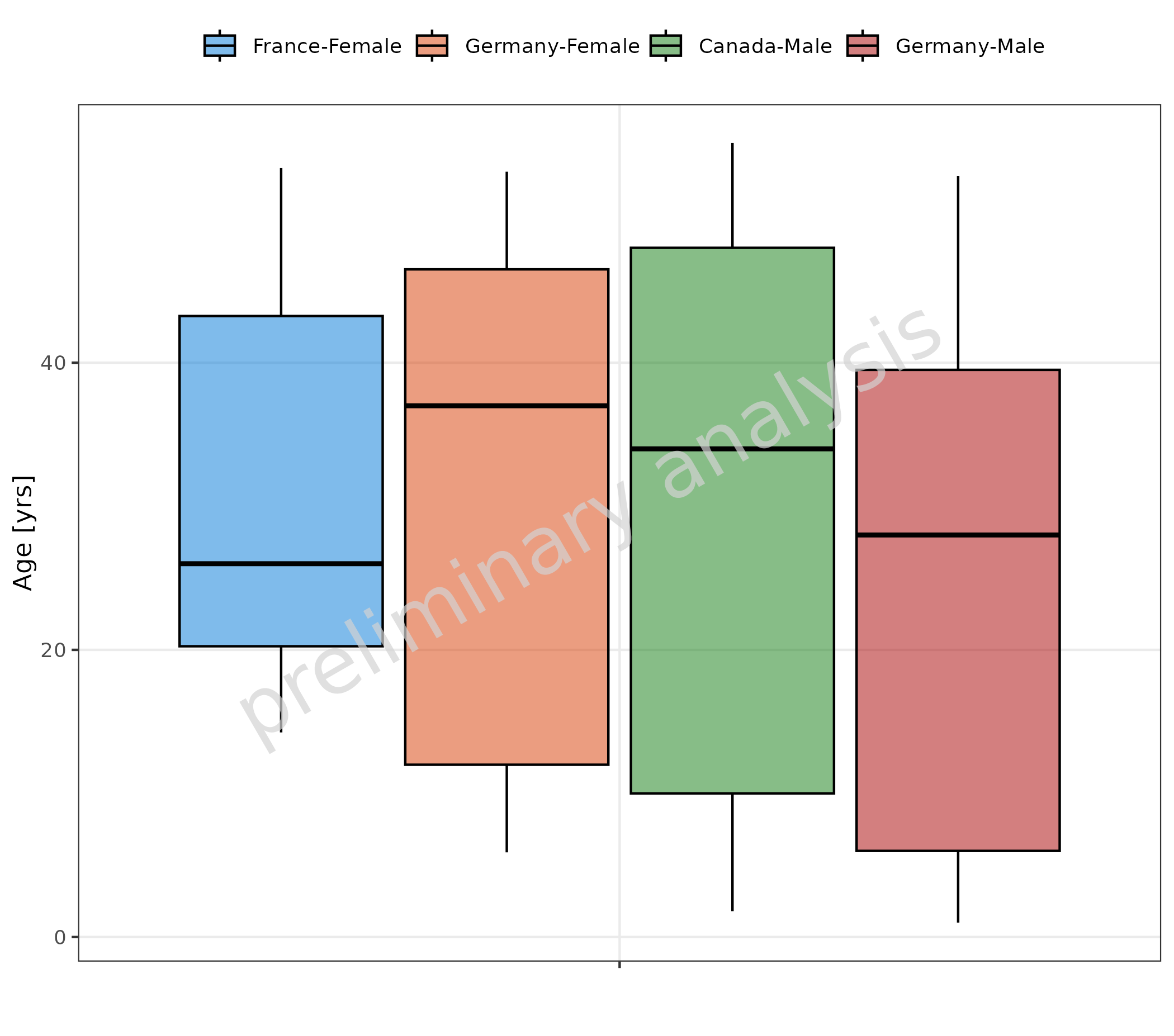

Box plot showing age distribution grouped by the interaction of country and sex. Each combination of country and sex is represented as a separate group with distinct colors in the legend.

2.1.6 Omit Data Points Flagged as Missing Dependent Variable (MDV)

If some of the data should be omitted, we can do this by mapping a logical column to the aesthetic mdv. Below, we exclude data from Germany:

plotBoxWhisker(
  mapping = aes(
    x = Country,
    y = Age,
    mdv = Country == "Germany",
    groupby = Sex
  ),
  data = pkRatioData,
  metaData = metaData
)

Box plots showing age distribution by country and sex, with data from Germany excluded using the missing dependent variable (MDV) flag. The plot demonstrates how to omit specific data points from the analysis.

2.2 Examples for Box-Whisker vs Numeric Data

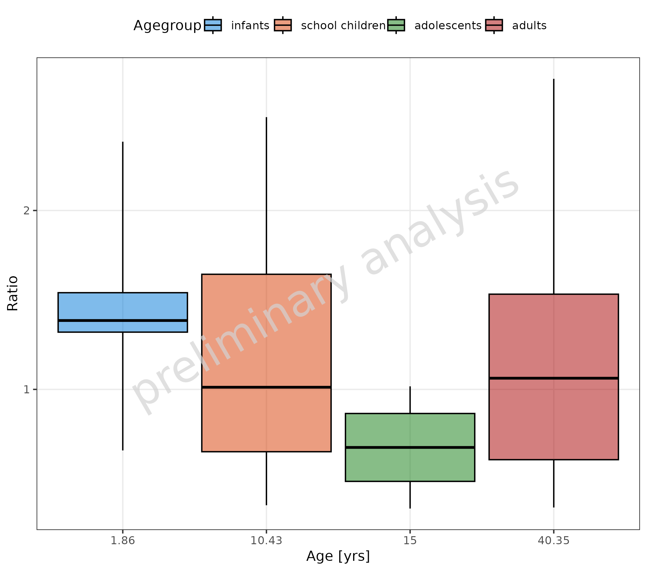
2.2.1 Numeric Data as Factor

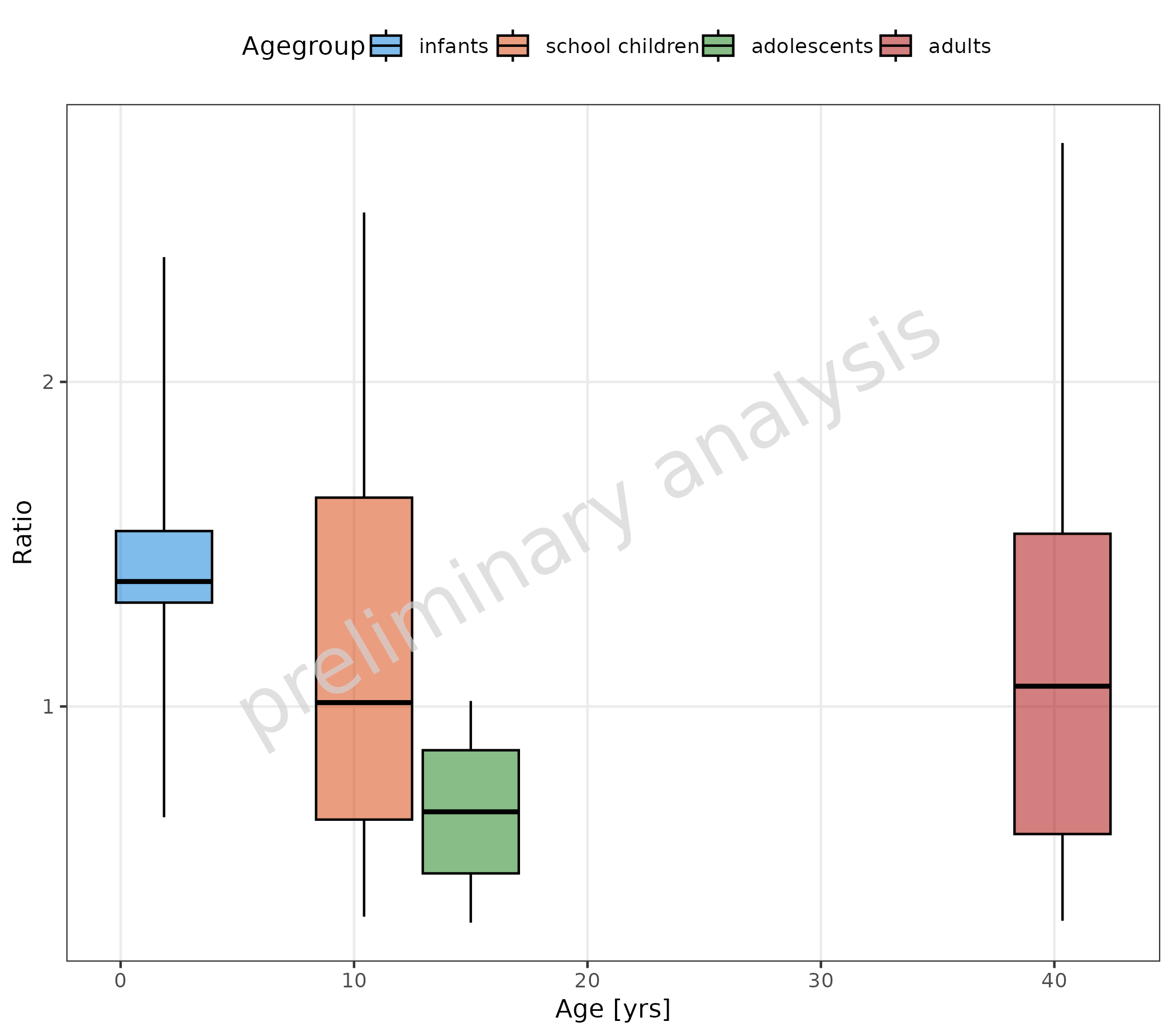
In the next example, we added a numeric column as “mean age” of the age group to the dataset. This column is mapped as factor to x. The values are now displayed as categorical values equidistant:

pkRatioData <- pkRatioData %>%
  dplyr::group_by(Agegroup) %>%
  dplyr::mutate(meanAge = round(mean(Age), 2))

metaData[["meanAge"]] <- metaData[["Age"]]
metaData <- metaData[intersect(names(pkRatioData), names(metaData))]

plotBoxWhisker(
  data = pkRatioData,
  mapping = aes(
    x = as.factor(meanAge),
    y = Ratio,
    fill = Agegroup
  ),
  metaData = metaData
)

Box plots showing ratio distribution by mean age treated as categorical factors. Each mean age value is positioned equidistantly on the x-axis, with different age groups represented by different fill colors.

2.2.2 Numeric Data as Distinct Numeric Values

If the column mapped to x is numeric and not a factor, the x-position of the boxes corresponds to the numeric value:

plotBoxWhisker(
  mapping = aes(
    x = meanAge,
    y = Ratio,
    fill = Agegroup
  ),
  data = pkRatioData,
  metaData = metaData
)

Box plots showing ratio distribution by mean age as continuous numeric values. The x-position of each box plot corresponds to its actual numeric mean age value, with different age groups represented by different fill colors.

2.2.3 Map Continuous Column with Binning

By mapping x with a function, it is possible to aggregate data of a continuous column into bins. Below, we use the function cut to aggregate the data into 4 distinct bins (see ?cut).

Attention: for cut(Age), no metaData exists. So we have to set the x label manually.

plotBoxWhisker(
  mapping = aes(
    x = cut(Age, 4),
    y = Ratio
  ),
  data = pkRatioData,
  metaData = metaData
) + labs(x = "Age range [years]")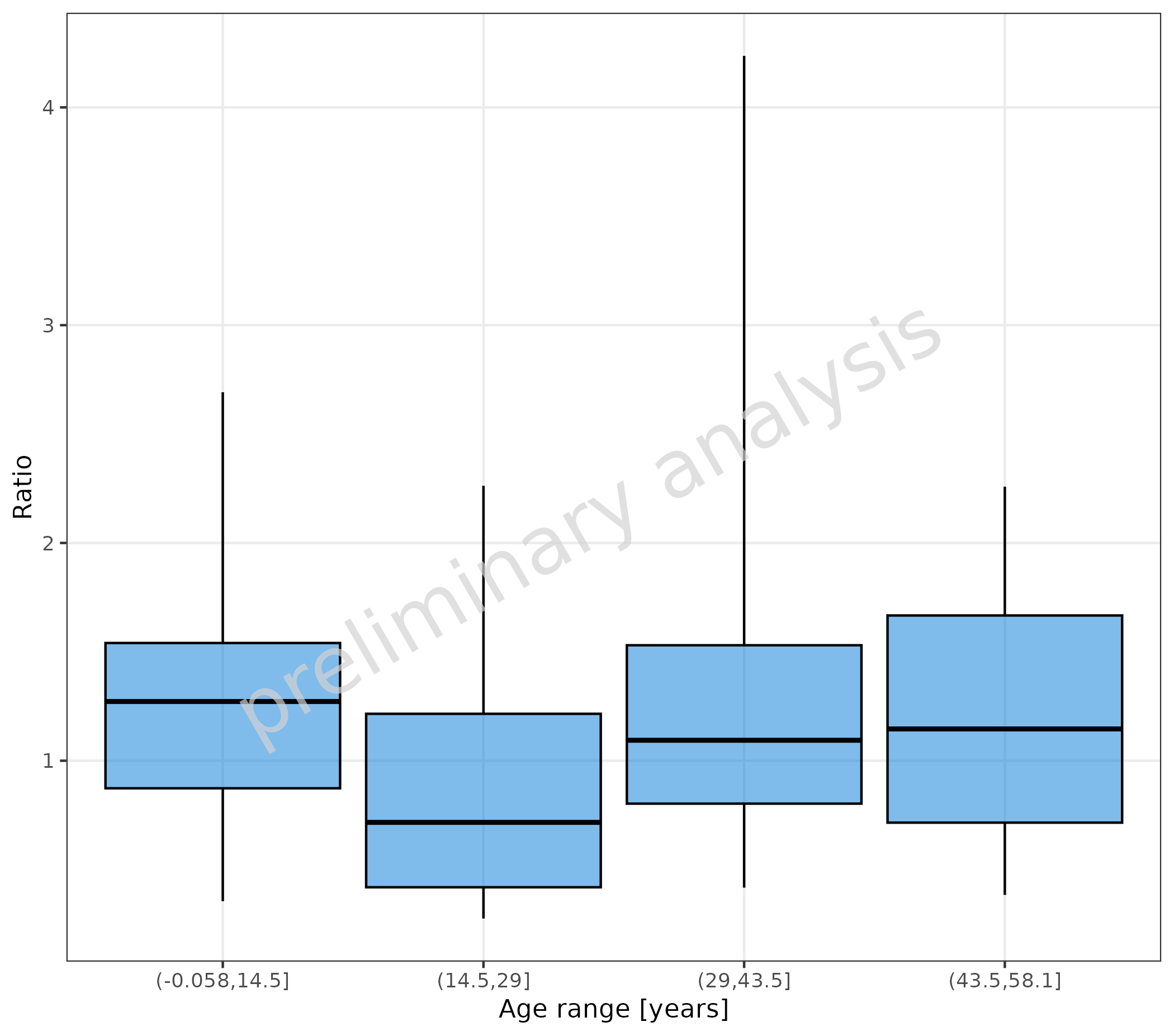

Box plots showing ratio distribution across four automatically generated age ranges. The continuous age variable is binned into four equal intervals, with each bin represented as a separate box plot on the x-axis.

We can use any function that converts a continuous vector to a factor. Below, we define our own cut function simply as a wrapper around cut, with some fixed arguments. This function is then mapped to x and groupby.

myCutfun <- function(x) {
  cut(x = x, breaks = c(0, 6, 12, 18, 60), include.lowest = TRUE, labels = c("infants", "school children", "adolescents", "adults"))
}

plotBoxWhisker(
  mapping = aes(
    x = myCutfun(Age),
    y = Ratio,
    groupby = myCutfun(Age)
  ),
  data = pkRatioData,
  metaData = metaData
) +
  theme(legend.title = element_blank()) +
  labs(x = "")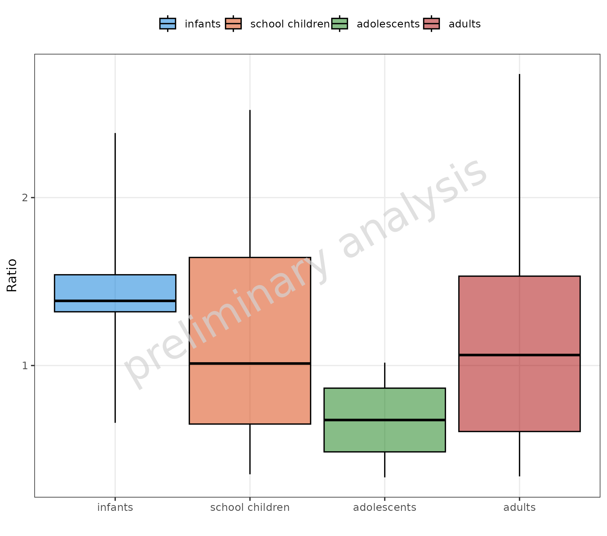

Box plots showing ratio distribution across predefined age groups using a custom binning function. Ages are categorized into infants, school children, adolescents, and adults, with each group shown as a separate box plot.

2.3 Aggregation Function

By default, the data is aggregated by percentiles defined by the default option ospsuite.plots.Percentiles. The percentiles can be customized for a specific plot by the input variable percentiles or for all plots generated by plotBoxWhisker() by changing the default options (setOspsuite.plots.option(optionKey = OptionKeys$Percentiles, value = c(0.05, 0.25, 0.5, 0.75, 0.95))).

It is also possible to use a customized function via the input variable statFun. If statFun is not NULL, it will overwrite the percentiles.

Important: If you override the defaults this way, please make sure to specify this in the plot annotations, as you are essentially redefining a box plot, and the reader might misinterpret it.

2.3.1 Example for Customized Percentiles

In the example below, we do not show the whiskers by setting whisker percentiles to box percentiles.

# B No whiskers
plotBoxWhisker(
  mapping = aes(
    x = Country,
    y = Age
  ),
  data = pkRatioData,
  metaData = metaData,
  percentiles = c(0.25, 0.25, 0.5, 0.75, 0.75)
)

Box plots showing age distribution by country with customized percentiles. The whiskers are removed by setting both whisker percentiles equal to the box percentiles, showing only the interquartile range.

2.3.2 Example for Customized Aggregation Function

To customize the aggregation, provide a function that has as input the vector to aggregate and as output a named list with entries ymin, lower, middle, upper, and ymax. In the example below, the function myStatFun is provided, which uses mean and standard deviation to aggregate:

myStatFun <- function(y) {
  r <- list(
    ymin = mean(y) - 1.96 * stats::sd(y),
    lower = mean(y) - stats::sd(y),
    middle = mean(y),
    upper = mean(y) + stats::sd(y),
    ymax = mean(y) + 1.96 * stats::sd(y)
  )
  return(r)
}

plotBoxWhisker(
  mapping = aes(
    x = Country,
    y = Age
  ),
  data = pkRatioData,
  metaData = metaData,
  statFun = myStatFun
) + labs(caption = "Mean for the middle line, mean +/- standard deviation for the box edges, and mean +/- 1.96 standard deviation for the whiskers.")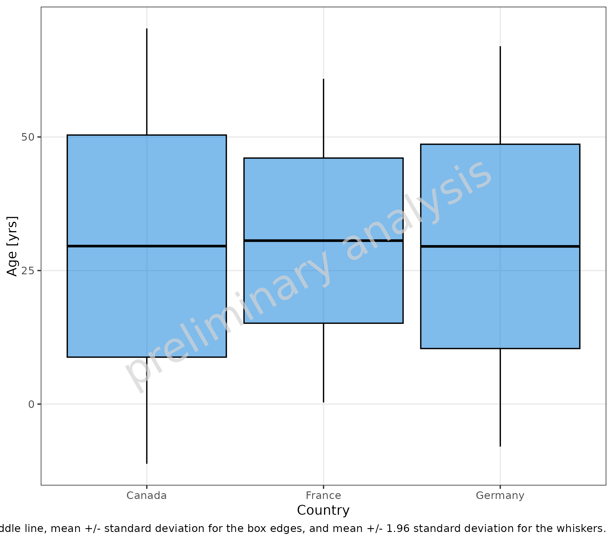

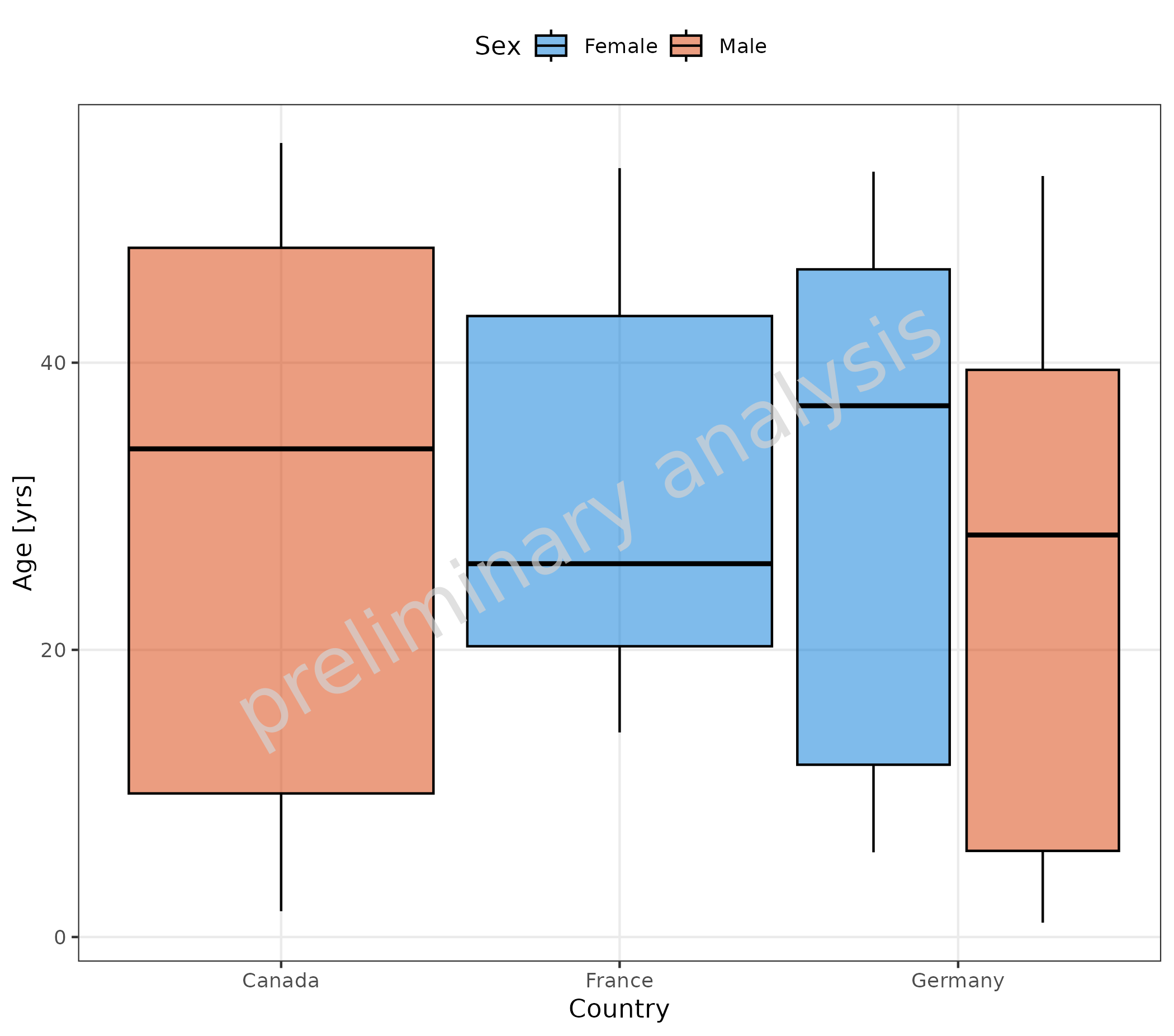
Box plots showing age distribution by country using a custom aggregation function based on mean and standard deviation. The middle line represents the mean, box edges show mean ± SD, and whiskers extend to mean ± 1.96 SD.

2.3.3 Tables Corresponding to Plot

As there already exist many possibilities to aggregate data in R, this package does not provide an extra function to return the aggregated data in a tabular form.

However, the plotBoxWhisker() adds the aggregation function to the plot object. So the aggregation can be easily done, e.g., with the data.table package using the same function as used for the plot.

# Generate plot object
plotObject <- plotBoxWhisker(
  mapping = aes(
    x = Country,
    y = Age,
    fill = Sex
  ),
  data = pkRatioData,
  metaData = metaData
)

plot(plotObject)

# Convert data to data.table and use statFun saved in plotObject for aggregation
# Make sure to add all relevant aesthetics to "by" columns
dt <- plotObject$data %>%
  data.table::setDT() %>%
  .[, as.list(plotObject$statFun(Age)), by = c("Country", "Sex")]

knitr::kable(dt)

Country	Sex	N	5th percentile	25th percentile	50th percentile	75th percentile	95th percentile	arith mean	arith standard deviation	arith CV	geo mean	geo standard deviation	geo CV
Canada	Male	19	1.80	10.00	34	48.00	55.30	29.57895	20.78813	0.7028014	0.00000	NaN	99.85178
Germany	Male	6	1.00	6.00	28	39.50	53.00	26.00000	22.54773	0.8672203	10.94354	6.561529	128.19570
Germany	Female	15	5.90	12.00	37	46.50	53.30	30.93333	18.25794	0.5902351	22.18088	2.949280	67.91401
France	Female	10	14.25	20.25	26	43.25	53.55	30.60000	15.45747	0.5051460	27.27291	1.662613	42.44874

Box plots showing age distribution by country and sex. This plot demonstrates how the aggregation function can be extracted from the plot object for creating corresponding data tables.

2.4 Show Outliers

2.4.1 Outliers with Default Settings

Outliers are displayed if the variable outliers is TRUE. Default outliers are flagged when outside the range from the “25th” percentile - 1.5 x IQR to the “75th” percentile + 1.5 x IQR.

plotBoxWhisker(
  mapping = aes(
    x = Sex,
    y = Ratio,
    fill = Country
  ),
  data = pkRatioData,
  metaData = metaData,
  outliers = TRUE
) + labs(tag = "A", caption = "Default settings: Whiskers indicate 90% range (5th - 95th percentile) and outliers indicate all measurements outside 25th percentiles - 1.5 x IQR to 75th percentiles + 1.5 x IQR.")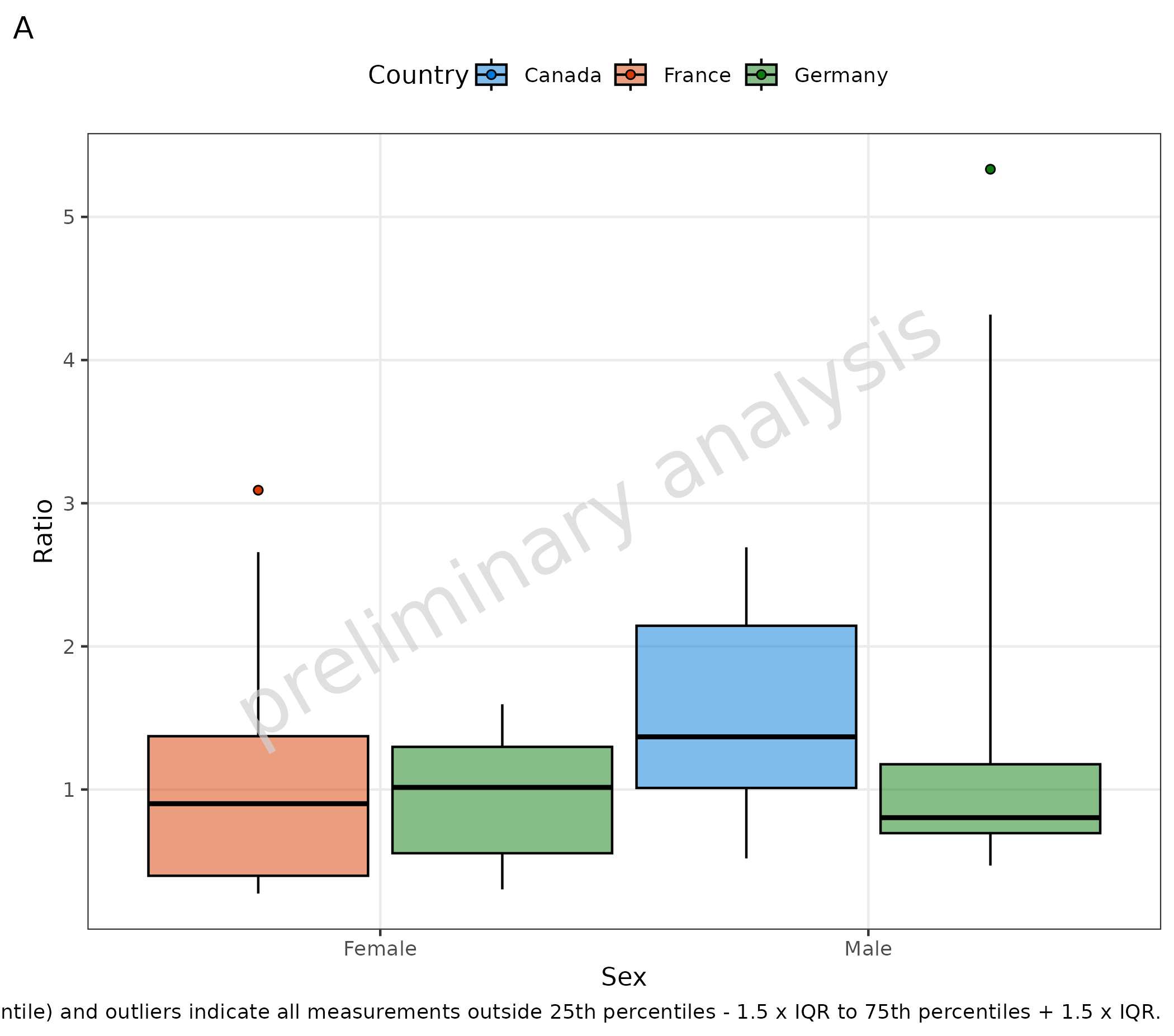

Box plots showing ratio distribution by sex and country with outliers displayed. Outliers are shown as individual points outside the whiskers, which indicate the 90% range (5th-95th percentile). Default outlier detection uses 1.5 × IQR beyond the quartiles.

2.4.2 Outliers with Customized Settings

In the following example, the aggregation is customized to set the whiskers to 10% and 90% via the input variable percentiles, and the outlier range is customized to show all points outside the whiskers. For that, we define a function myStatFunOutlier, which has as input the vector of the values and as output the vector of values outside the outlier range.

myStatFunOutlier <- function(y) {
  q <- stats::quantile(y, probs = c(0.1, 0.9), names = FALSE, na.rm = TRUE)
  yOutsideRange <- subset(y, y < q[1] | y > q[2])

  if (length(yOutsideRange) < 1) {
    return(as.double(NA))
  } else {
    return(yOutsideRange)
  }
}

plotBoxWhisker(
  data = pkRatioData,
  metaData = metaData,
  mapping = aes(
    x = Sex,
    y = Ratio,
    fill = Country
  ),
  outliers = TRUE,
  percentiles = c(0.1, 0.25, 0.5, 0.75, 0.9),
  statFunOutlier = myStatFunOutlier
) + labs(caption = "Whiskers indicate 80% range (10th - 90th percentile) and outliers indicate all measurements outside whiskers.")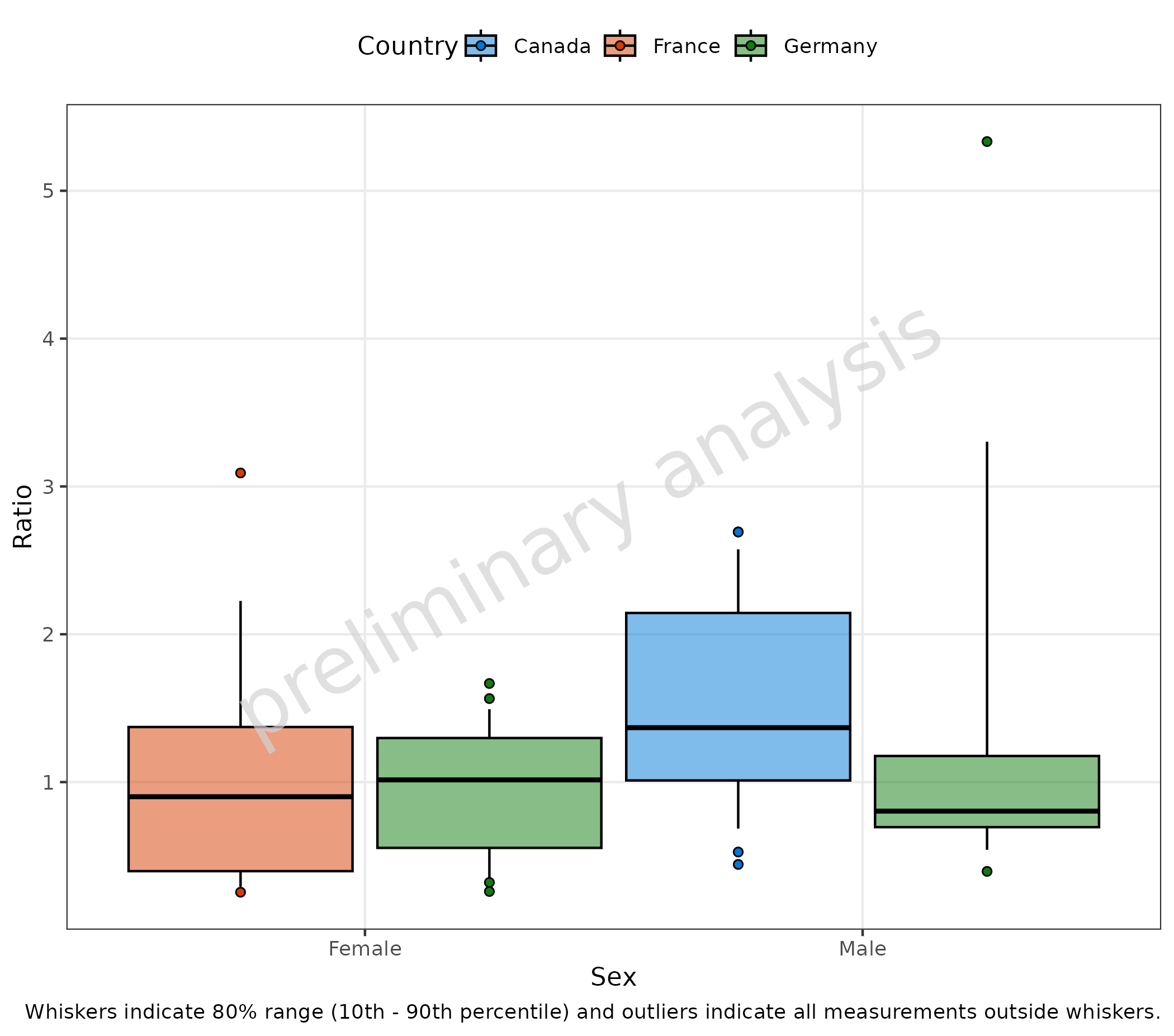

Box plots showing ratio distribution by sex and country with custom outlier detection. The whiskers indicate the 80% range (10th-90th percentile), and outliers show all measurements outside the whisker range.

2.4.3 Retrieve Outliers as Table

The plotBoxWhisker() adds the outlier function to the plot object. So outliers can be easily retrieved, e.g., with the data.table package.

# Generate plotObject
plotObject <- plotBoxWhisker(
  data = pkRatioData,
  metaData = metaData,
  mapping = aes(
    x = Sex,
    y = Ratio,
    fill = Country
  ),
  outliers = TRUE,
  percentiles = c(0.1, 0.25, 0.5, 0.75, 0.9),
  statFunOutlier = myStatFunOutlier
)

# Convert data to data.table and use statFun saved in plotObject for aggregation
# Make sure to add all relevant aesthetics to "by" columns
dt <- plotObject$data %>%
  data.table::setDT() %>%
  .[, .(outliers = plotObject$statFunOutlier(Ratio)), by = c("Country", "Sex")]

knitr::kable(dt)

Country	Sex	outliers
Canada	Male	2.692
Canada	Male	0.443
Canada	Male	2.692
Canada	Male	0.527
Germany	Male	5.333
Germany	Male	0.396
Germany	Female	1.667
Germany	Female	1.565
Germany	Female	0.260
Germany	Female	0.321
France	Female	3.091
France	Female	0.255

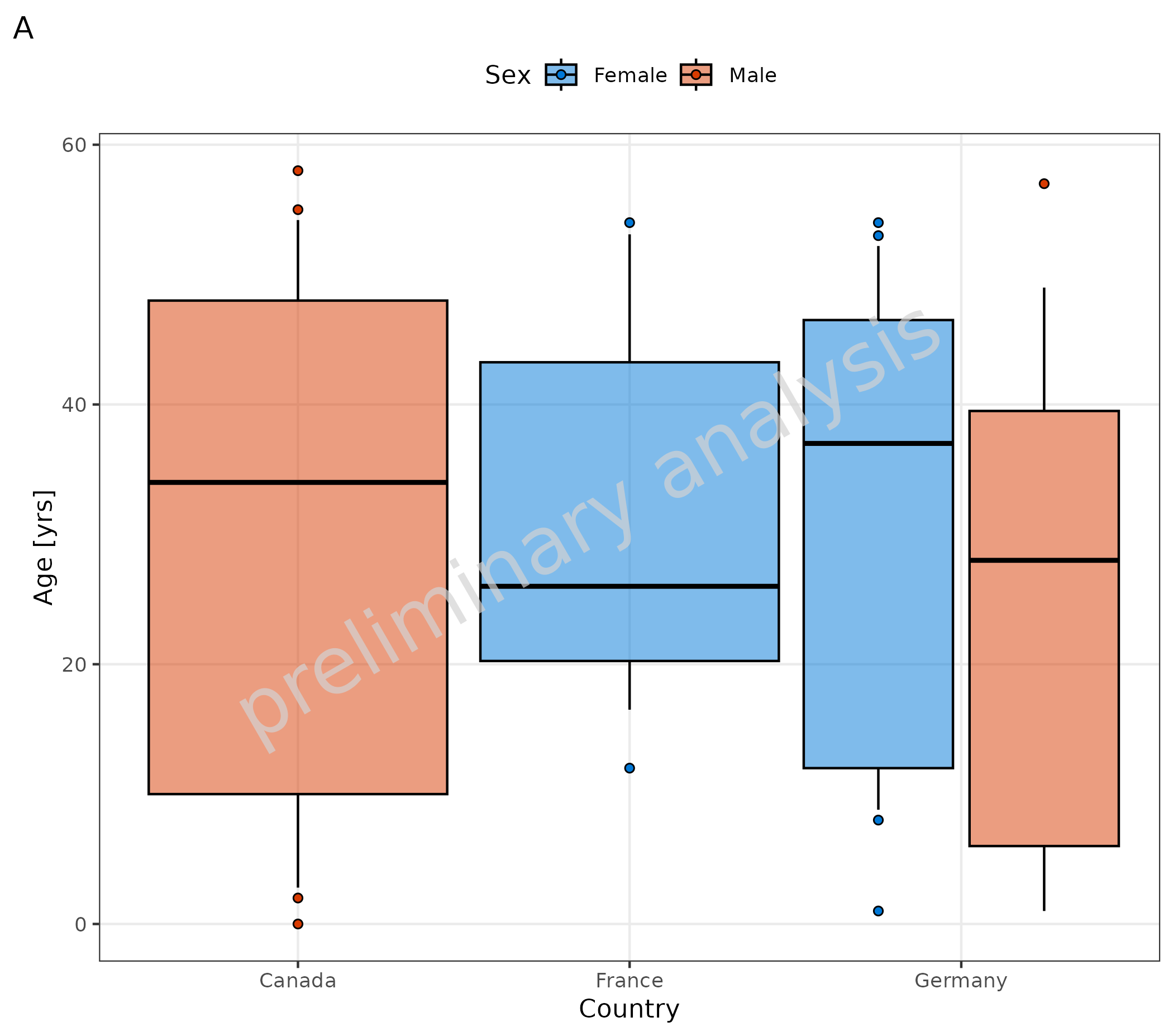
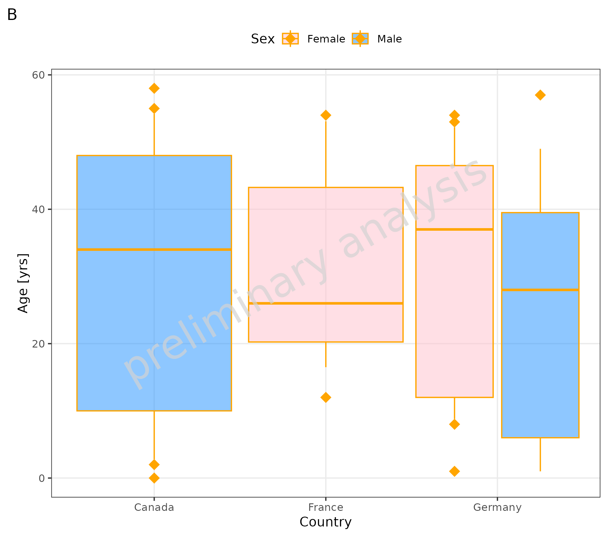
3. Plot Configuration of Boxplots

Below you see an example of the same plot:

A default layout
B customized layout
The variable geomBoxplotAttributes now has an entry for color ‘orange’.
The variable geomPointAttributes now has an entry for size = 4, color ‘orange’, and shape = ‘diamond’.
Fill is added to the mapping, so the outlier points are also colored according to ‘Sex’.
With scale_fill_manual, the colors for ‘Sex’ are defined.

# A default layout
plotBoxWhisker(
  data = pkRatioData,
  metaData = metaData,
  mapping = aes(
    x = Country,
    y = Age,
    fill = Sex
  ),
  outliers = TRUE,
  percentiles = c(0.1, 0.25, 0.5, 0.75, 0.9),
  statFunOutlier = myStatFunOutlier
) + labs(tag = "A")

# B customized layout
plotBoxWhisker(
  data = pkRatioData,
  metaData = metaData,
  mapping = aes(
    x = Country,
    y = Age,
    fill = Sex
  ),
  outliers = TRUE,
  percentiles = c(0.1, 0.25, 0.5, 0.75, 0.9),
  statFunOutlier = myStatFunOutlier,
  geomBoxplotAttributes = list(color = "orange", position = position_dodge(width = 1)),
  geomPointAttributes = list(position = position_dodge(width = 1), size = 4, color = "orange", shape = "diamond")
) + scale_fill_manual(values = c(Female = "pink", Male = "dodgerblue")) + labs(tag = "B")

Two side-by-side box plots (A and B) showing age distribution by country and sex. Plot A shows default styling, while Plot B demonstrates custom styling with orange colors for boxes and diamond-shaped outlier points, plus custom fill colors for sex groups.