Mathematical overview of variance-based methods

This article provides a mathematical overview of the variance-based global sensitivity analysis methods implemented in the OSP Global Sensitivity package, namely the Sobol method of Homma & Saltelli and the Extended Fourier Amplitude Sensitivity Test (EFAST) method of Saltelli et al. It corresponds to Supplementary Materials 2 of the accompanying publication:

Najjar A, Hamadeh A, Krause S, Schepky A, Edginton A. Global sensitivity analysis of Open Systems Pharmacology Suite physiologically based pharmacokinetic models. CPT Pharmacometrics Syst Pharmacol. 2024;13:2052-2067. doi: 10.1002/psp4.13256

Variance-based methods start by expressing a pharmacokinetic parameter $PK$ in terms of a summation of functions of subsets of the parameters $p_{1},\cdots,\ p_{n}$, as described in Homma & Saltelli:

$$PK = h\left( p_{1},\cdots,p_{n} \right) = h_{0} + \sum_{i} h_{i}\left( p_{i} \right) + \sum_{i,j} h_{ij}\left( p_{i},\ p_{j} \right) + \cdots + h_{1\cdots n}\left( p_{1},\cdots,\ p_{n} \right) \quad (1)$$

Thus, the decomposition of Equation 1 splits $PK$ into distinct functions corresponding to each unique combination of parameters $p_{1}\cdots p_{n}$. The variance $D$ of $PK$ may similarly be decomposed. For the case of $n = 3$ parameters ($p_{1}$, $p_{2}$, $p_{3}$), the decomposition of the total variance is as follows:

$$D = D_{1} + D_{2} + D_{3} + D_{12} + D_{13} + D_{23} + D_{123}$$

The indices $D_{i}$ represent first order indices that quantify the proportion of the total variance $D$ that is due to variation solely in a single parameter $p_{i}$. In addition, as defined in Homma & Saltelli, a total effect $D_{i}^{T}$ can also be defined as the sum of all components of $Var(PK)$ that involve parameter $i$. For the case of $n = 3$ parameters, the total effect variances are given by

$$D_{1}^{T} = D_{1} + D_{12} + D_{13} + D_{123} = D - D_{2} - D_{3} - D_{23}$$$$D_{2}^{T} = D_{2} + D_{12} + D_{23} + D_{123} = D - D_{1} - D_{3} - D_{13}$$$$D_{3}^{T} = D_{3} + D_{13} + D_{23} + D_{123} = D - D_{1} - D_{2} - D_{12}$$

The first order sensitivity for parameter $p_{i}$ is thus given by $S_{i} = D_{i}/D$, and the corresponding total effect sensitivity $S_{i}^{T} = D_{i}^{T}/D$.

Mathematical derivation

The decomposition of $PK$ in terms of a summation of functions of subsets of the parameters $p_{1},\cdots,\ p_{n}$, as given in Equation 1, is such that, by construction,

$$\int h_{i\cdots j}\left( p_{i},\cdots,p_{j} \right)P\left( p_{i},\cdots,p_{j} \right)dp_{k} = 0 \quad \text{for any } k \in i,\cdots,j. \quad (2)$$

Without loss of generality, we limit this analysis to the case $n = 3$, and therefore:

$$h = h_{0} + h_{1} + h_{2} + h_{3} + h_{12} + h_{13} + h_{23} + h_{123}$$

The function $h\left( p_{1},p_{2},p_{3} \right)$ has mean value

$$h_{0} = E\lbrack PK\rbrack = \int h(p_{1},p_{2},p_{3}) \cdot P\left( p_{1},p_{2},p_{3} \right) \cdot dp_{1}dp_{2}dp_{3}$$

Under the condition of Equation 2,

$$\int h_{123}\left( p_{1},p_{2},p_{3} \right)P\left( p_{1},p_{2},p_{3} \right)dp_{2}dp_{3} = 0 = \int h\left( p_{1},p_{2},p_{3} \right) \cdot P\left( p_{1},p_{2},p_{3} \right)dp_{2}dp_{3} - h_{0} - h_{1}$$

Yielding $h_{1}\left( p_{1} \right) = E\left\lbrack PK|p_{1} \right\rbrack - h_{0}$, and similarly $h_{2}\left( p_{2} \right) = E\left\lbrack PK|p_{2} \right\rbrack - h_{0}$ and $h_{3}\left( p_{3} \right) = E\left\lbrack PK|p_{3} \right\rbrack - h_{0}$.

Similarly, using Equation 1,

$$\int h_{123}\left( p_{1},p_{2},p_{3} \right)P\left( p_{1},p_{2},p_{3} \right)dp_{1} = 0 = \int h\left( p_{1},p_{2},p_{3} \right) \cdot P\left( p_{1},p_{2},p_{3} \right)dp_{1} - h_{0} - h_{2} - h_{3} - h_{23}$$

which yields $h_{23}\left( p_{2},p_{3} \right) = E\left\lbrack PK|p_{2},p_{3} \right\rbrack - h_{0} - h_{2} - h_{3}$, and similarly $h_{12}\left( p_{1},p_{2} \right) = E\left\lbrack PK|p_{1},p_{2} \right\rbrack - h_{0} - h_{1} - h_{2}$ and $h_{13}\left( p_{1},p_{3} \right) = E\left\lbrack PK|p_{1},p_{3} \right\rbrack - h_{0} - h_{1} - h_{3}$.

Moreover, as shown in Homma & Saltelli, any two (distinct) functions $h_{i\cdots j}$ and $h_{i'\cdots j'}$ are orthogonal:

$$\int h_{i\cdots j}\left( p_{i},\cdots,\ p_{j} \right) \cdot h_{i'\cdots j'}\left( p_{i'},\cdots,\ p_{j'} \right) \cdot P\left( p_{1},\cdots,\ p_{n} \right)\ dp_{1}\cdots dp_{n} = 0$$

Based on this decomposition and the orthogonality property, the variance of $PK$ may also be decomposed. For the case of $n = 3$ parameters, the total variance in the PK parameter ($Var(PK)$) is decomposed as

$$Var(PK) = D = D_{1} + D_{2} + D_{3} + D_{12} + D_{13} + D_{23} + D_{123}$$

where

$$D_{i\cdots j} = \int h_{i\cdots j}^{2}\left( p_{i},\cdots,p_{j} \right) \cdot P\left( p_{i},\cdots,p_{j} \right) \cdot dp_{i}\cdots dp_{j}$$

The first order effect is given by

$$D_{i} = Var\left\lbrack E\left\lbrack PK|p_{i} \right\rbrack \right\rbrack = \int h_{i}^{2}\left( p_{i} \right) \cdot P\left( p_{i} \right) \cdot dp_{i} = \int \left( \int h\left( p_{1},\cdots,\ p_{n} \right) \cdot P\left( p_{j \neq i} \right) \cdot dp_{j \neq i} \right)^{2} \cdot P\left( p_{i} \right) \cdot dp_{i} - f_{0}^{2} \quad (3)$$

while the total effect is given by

$$D_{i}^{T} = Var(PK) - Var\left( E\lbrack PK|p_{j \neq i}\rbrack \right) = \int h^{2}\left( p_{1},\cdots,p_{n} \right) \cdot P\left( p_{1},\cdots,p_{n} \right) \cdot dp_{1}\cdots dp_{n} - \int \left( \int h\left( p_{1},\cdots,p_{n} \right) \cdot P\left( p_{i} \right) \cdot dp_{i} \right)^{2} \cdot P\left( p_{j \neq i} \right) \cdot dp_{j \neq i} \quad (4)$$

For the case of $n = 3$ parameters, the total effect variances are given by

$$D_{1}^{T} = D_{1} + D_{12} + D_{13} + D_{123} = D - D_{2} - D_{3} - D_{23} = Var(PK) - Var\left( E\lbrack PK|p_{2},p_{3}\rbrack \right) \quad (5)$$$$D_{2}^{T} = D_{2} + D_{12} + D_{23} + D_{123} = D - D_{1} - D_{3} - D_{13} = Var(PK) - Var\left( E\lbrack PK|p_{1},p_{3}\rbrack \right)$$$$D_{3}^{T} = D_{3} + D_{13} + D_{23} + D_{123} = D - D_{1} - D_{2} - D_{12} = Var(PK) - Var\left( E\lbrack PK|p_{1},p_{2}\rbrack \right)$$

The first order sensitivity for parameter $p_{i}$ is thus given by $S_{i} = D_{i}/D$, and the corresponding total effect sensitivity $S_{i}^{T} = D_{i}^{T}/D$.

Computation of variance-based sensitivity indices

The computation of the first order and total effect indices requires evaluating the $PK$ of the model outputs $y(t)$ at numerous points in the space of parameters $p_{1},\cdots,p_{n}$. A variety of methods have been reported for efficiently traversing this parameter space in a way that gives satisfactory evaluation of $S_{i}$ and $S_{i}^{T}$. The OSP Global Sensitivity package provides two methods for sampling the parameter space and computing $S_{i}$ and $S_{i}^{T}$: that of Homma & Saltelli and the EFAST method in Saltelli et al.

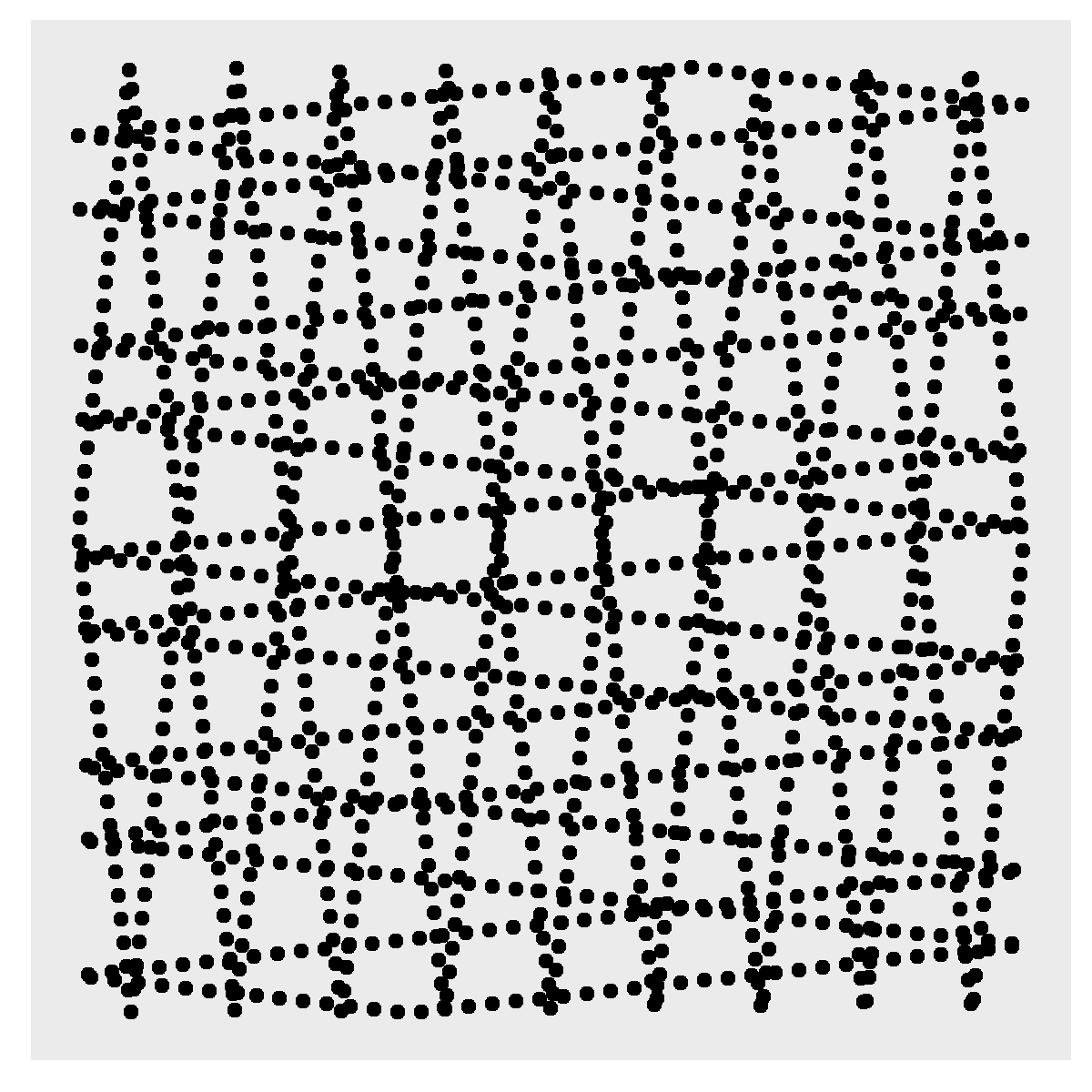
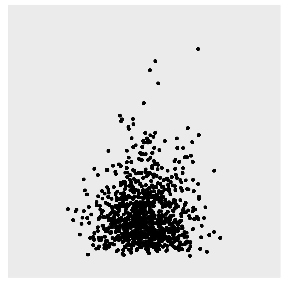
The initial stage in both methodologies entails the establishment of a sampling scheme for the selection of points within the parameter space where $PK$ is to be evaluated. One possibility is to use a uniform distribution over the unit hypercube of quantiles of the probability distribution of the parameters $p_{1},\cdots,\ p_{n}$. The inverse cumulative probability distribution of each parameter can then be used to map the point in the quantile space to the corresponding point in the parameter space for input into the PBPK model (Figure 1-A). Alternative methods are however used in both Homma & Saltelli and the EFAST method in Saltelli et al., as described next.

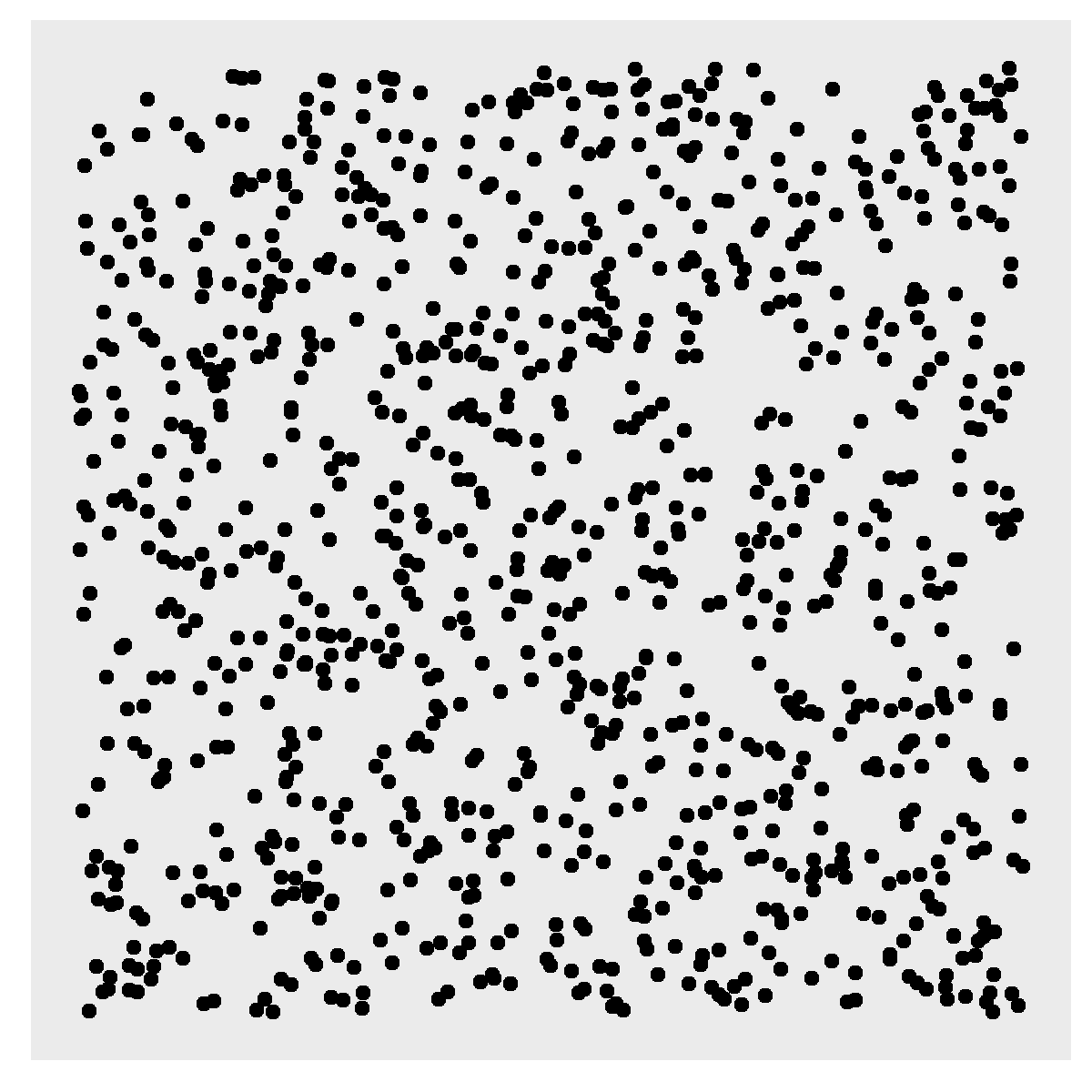
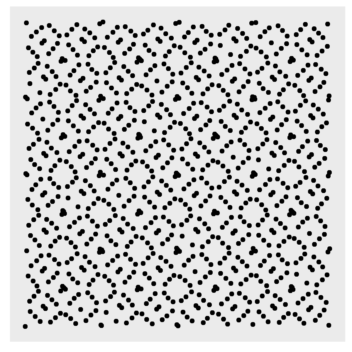
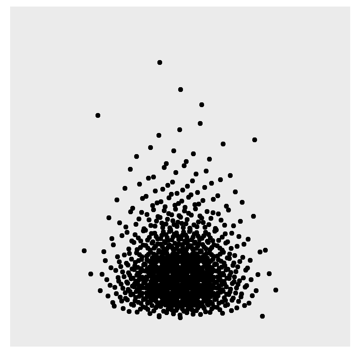
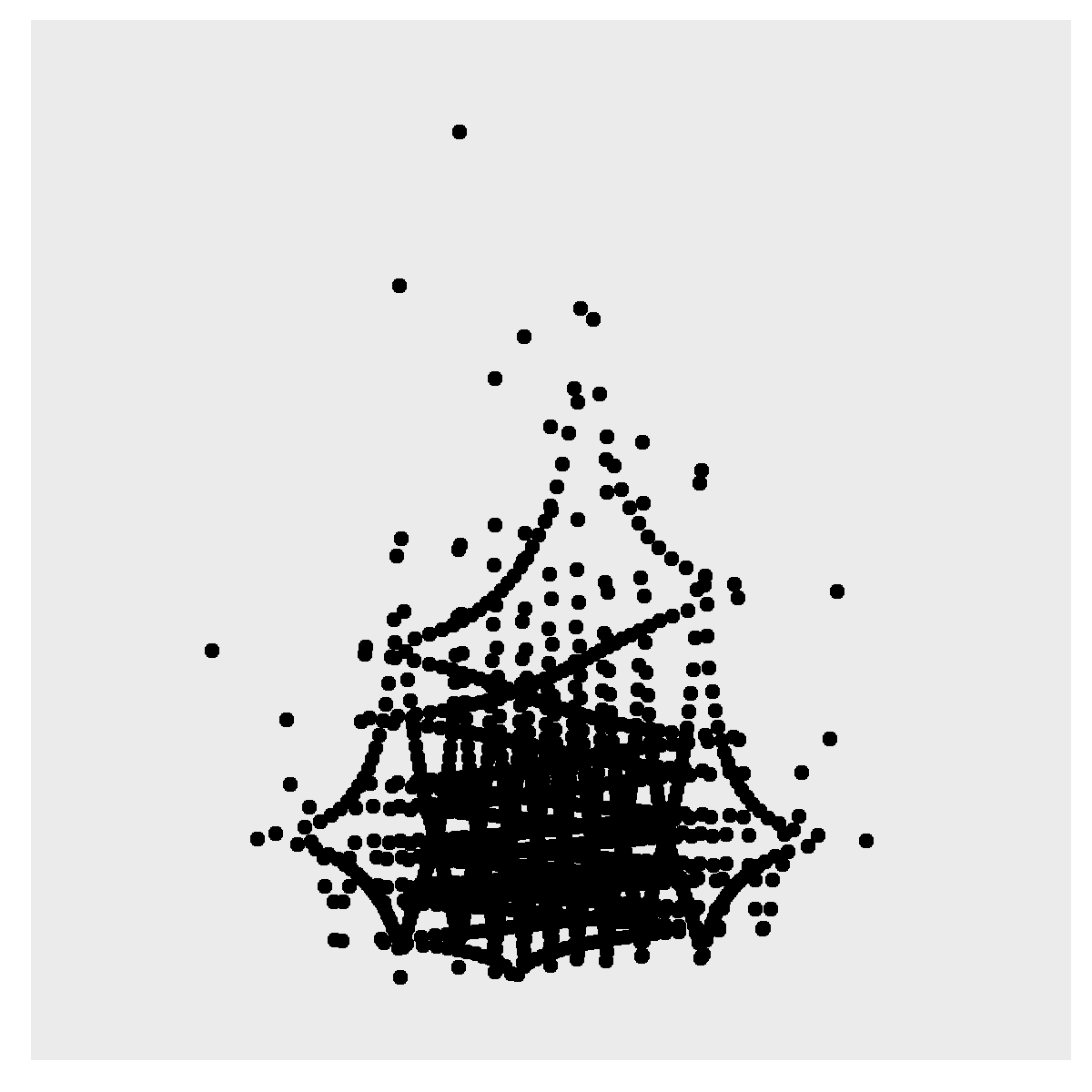
Figure 1. Sampling strategies on the unit square of quantiles (left of each pair) and their translation onto parameter space (right of each pair) under (A) uniform sampling, (B) Sobol sequence sampling, and (C) EFAST sampling.

Homma & Saltelli (Sobol)

The sampling of the parameter space in Homma & Saltelli utilizes a Sobol quasi-random Monte Carlo method. As shown in Figure 1-B, this approach offers the advantage of producing more evenly distributed and less clustered points across the unit hypercube compared to uniform sampling, while maintaining a quasi-random distribution.

To compute the sensitivity indices $S_{i}$ and $S_{i}^{T}$, the following procedure from Homma & Saltelli is used. Two sets of Sobol sequences of $N$ samples (where $N$ is user-selected) from the unit $n$-dimensional hypercube are generated and then mapped into the parameter space via the inverse cumulative distributions of the parameters $P(p_{i})$. These parameter space samples can be organized into $N \times n$ matrices, which we denote by $U_{A}$ and $U_{B}$. For the case of $n = 3$ parameters, these can be represented as

$$U_{A} = \begin{bmatrix} \vdots & \vdots & \vdots \\ A_{1} & A_{2} & A_{3} \\ \vdots & \vdots & \vdots \end{bmatrix} \quad \text{and} \quad U_{B} = \begin{bmatrix} \vdots & \vdots & \vdots \\ B_{1} & B_{2} & B_{3} \\ \vdots & \vdots & \vdots \end{bmatrix}$$

A total of $n$ additional sets of samples ($U_{1},\ \cdots,U_{n}$) are then generated from the original two by substituting columns from $U_{A}$ into $U_{B}$. For the case of $n = 3$ parameters:

$$U_{1} = \begin{bmatrix} \vdots & \vdots & \vdots \\ A_{1} & B_{2} & B_{3} \\ \vdots & \vdots & \vdots \end{bmatrix}, \quad U_{2} = \begin{bmatrix} \vdots & \vdots & \vdots \\ B_{1} & A_{2} & B_{3} \\ \vdots & \vdots & \vdots \end{bmatrix}, \quad U_{3} = \begin{bmatrix} \vdots & \vdots & \vdots \\ B_{1} & B_{2} & A_{3} \\ \vdots & \vdots & \vdots \end{bmatrix}$$

The PBPK model is evaluated with parameters $p_{1},\cdots,p_{n}$ set to the values in each of the $N$ rows of the $n + 2$ matrices $U_{A}$, $U_{B}$, and $U_{1},\cdots,U_{n}$, giving a total of $N(n + 2)$ model evaluations in each run of this algorithm.

The mean value of $PK$ is approximated by $h_{0} = \frac{1}{N}\sum_{j = 1}^{N} h\left( {U_{A}}_{j} \right)$, where $h\left( {U_{A}}_{j} \right)$ means that $PK = h\left( p_{1},\cdots,p_{n} \right)$ is evaluated using the parameters taken from the $j^{th}$ row of $U_{A}$.

Similarly, the total variance in $PK$ is estimated as $D = Var(PK) = \left( \frac{1}{N}\sum_{j = 1}^{N} h^{2}\left( {U_{A}}_{j} \right) \right) - h_{0}^{2}$, while the numerical approximation to the first order variance $D_{i}$ in Equation 3 is given by

$$D_{i} = \left( \frac{1}{N}\sum_{j = 1}^{N} h\left( {U_{A}}_{j} \right)h\left( {U_{i}}_{j} \right) \right) - h_{0}^{2}.$$

On the other hand, the total effect variance is approximated numerically as:

$$D_{i}^{T} = D - \left( \left( \frac{1}{N}\sum_{j = 1}^{N} h\left( {U_{B}}_{j} \right)h\left( {U_{i}}_{j} \right) \right) - h_{0}^{2} \right).$$

EFAST

In contrast to the Monte Carlo approach of Homma & Saltelli, the Extended Fourier Amplitude Sensitivity Test (EFAST) method of Saltelli et al. uses a systematic algorithm to traverse the space of parameters $p_{1},\cdots,\ p_{n}$ via a series of curves that oscillate periodically at different frequencies ($\omega_{1},\ \cdots,\omega_{n}$), as shown in Figure 2.

As the scalar $\theta$ varies from $\theta = 0$ to $\theta = 2\pi$, points in the $n$-dimensional hypercube are sampled along curves given by $\frac{1}{2} + \frac{1}{\pi}\arcsin\left( \sin\left( \omega_{i}\theta + \varphi_{i} \right) \right)$, where $\varphi_{i}$ is a random perturbation. The rate of sampling is given by $\omega_{s} = 2 \cdot M \cdot \omega_{\max} + 1$, where $\omega_{\max} = \max\left( \omega_{1},\ \cdots,\omega_{n} \right)$ and $M = 4$. Selection of the frequencies $\omega_{1},\ \cdots,\omega_{n}$ is as per Saltelli et al. The choice of $M$ and the sampling rate $\omega_{s}$ ensures adherence to the Nyquist sampling criterion, which requires the sampling rate of a signal (i.e., the $PK$ values as they vary in response to periodic variations in $p_{1},\cdots,p_{n}$) to be at least $2 \cdot \omega_{\max}$ to ensure no information loss and accurate reconstruction of the original signal from the acquired $PK$ samples.

The sampled points, residing in the quantile space within the unit hypercube, are mapped onto parameter space using the inverse cumulative distribution functions of the respective parameters $\left( p_{1},\cdots,\ p_{n} \right)$ (Figure 1-C). Evaluation of PK parameters such as $AUC$ and $C_{\max}$ is performed at each sample point by updating the PBPK model with the sample point values of $\left( p_{1},\cdots,\ p_{n} \right)$, simulating the model to evaluate the output time profile of interest ($y(t)$), and calculating the PK parameter for that output time profile.

To analyze the frequency characteristics of the resulting PK parameter evaluations, the Fast Fourier Transform (FFT) is employed (Figure 2). The FFT derives the frequency spectrum of the PK parameter as it varies across the sample point curves. First-order sensitivity indices of parameter $p_{i}$, $S_{1}\left( p_{i} \right)$, are calculated by assessing the fraction of the total spectrum at frequency $\omega_{i}$, which is associated with parameter $p_{i}$. Higher order harmonics (at frequencies ${2\omega}_{i},\ 3\omega_{i}, \cdots$) quantify interactions between parameter $p_{i}$ and other parameters. The total effect sensitivity indices $S_{1}^{T}\left( p_{i} \right)$ are computed by subtracting from the spectrum all frequency components that are not associated with parameter $p_{i}$ at frequencies ($\omega_{i},{2\omega}_{i},\ 3\omega_{i}, \cdots$).

For each model parameter $p_{i}$, the EFAST method in the OSP Global Sensitivity package evaluates $S_{1}\left( p_{i} \right)$ and $S_{1}^{T}\left( p_{i} \right)$ by setting a high frequency $\omega_{i}$ and a lower set of frequencies for the remaining parameters, thereby ensuring separation of the spectra associated with these parameters in the frequency space. The spectrum at $\omega_{i}$ and its higher order harmonics may then be separated from the spectrum associated with the remaining parameters $p_{j \neq i}$. This procedure is repeated $n$ times, once for each parameter. The user may specify the number of repetitions $N_{r} \geq 1$ of the algorithm, the results of which are averaged whenever $N_{r} > 1$. Thus, there are a total of $n \cdot N_{r} \cdot \left( 2 \cdot M \cdot \omega_{\max} + 1 \right)$ points at which the PBPK model is simulated and its PK parameters evaluated.

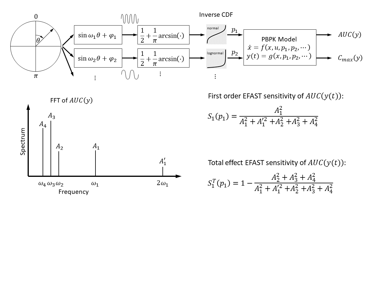
Figure 2. Overview of the EFAST global sensitivity method of Saltelli et al. The unit hypercube of quantiles is traversed via periodic curves of varying frequencies that correspond to model parameters as the scalar quantity theta varies over [0, 2*pi). Sampled points are mapped onto the space of parameters via the inverse cumulative distribution of each parameter, the PK parameters of interest are evaluated at each sample point, and the Fast Fourier Transform is used to derive the frequency spectrum of the resulting PK parameter evaluations.

References

1. Homma T, Saltelli A. Importance measures in global sensitivity analysis of nonlinear models. Reliability Engineering & System Safety. 1996;52:1-17.
2. Saltelli A, Tarantola S, Chan KP-S. A Quantitative Model-Independent Method for Global Sensitivity Analysis of Model Output. Technometrics. 1999;41(1):39-56.